How to Use apeglm and ashr for DESeq2 Shrinkage
By Dr. Zubair Khalid, DVM, MS, PhD ·

apeglm shrinks each DESeq2 fold change toward zero with an adaptive heavy-tailed prior and reports the posterior estimate for one named coefficient, while ashr fits a flexible mixture prior per gene and additionally supports arbitrary contrasts, nonzero thresholds, and s-values. The rule of thumb is simple. If you are analyzing a straightforward two-group design and can name your coefficient, use apeglm. If you need a contrast that is not a single coefficient, want to screen against a nonzero fold-change threshold, or work with interaction terms, use ashr. For most published two-group comparisons the two estimators give very similar shrunken log2 fold changes and the same biological conclusions, so the choice matters more for complex designs and threshold-based workflows than for a plain tumor versus normal contrast.
This guide covers the reasoning behind shrinkage, runnable code for both estimators, a side-by-side comparison of the practical options, worked scenarios, and a troubleshooting section for the error messages that come up most often in real RNA-seq projects.
Why DESeq2 Shrinks Fold Changes at All
Raw maximum likelihood estimates (MLEs) of log2 fold change are noisy for low-count genes. A gene with 8 total counts across all samples can show an observed fold change of 10 simply because tiny denominators amplify random variation. On an MA plot these genes form the characteristic funnel at the left edge, and they dominate naive rankings by effect size.
Shrinkage solves this by combining each gene's observed effect with a prior expectation that most genes have small or zero effects. The result is an empirical Bayes posterior estimate. Strongly supported effects barely move. Weakly supported effects collapse toward zero, which is exactly the behavior you want for ranking and visualization.
The DESeq2 package, maintained on Bioconductor by Michael Love, Wolfgang Huber, and Simon Anders, formalized this in two stages. Earlier versions applied a normal prior inside the main DESeq() call. Since DESeq2 version 1.16, the main fit estimates unshrunken MLE coefficients and Wald statistics, and shrinkage happens separately through the lfcShrink() function. Recent versions of the package default to apeglm as the shrinkage method. The lfcShrink() interface then accepts several estimators, of which apeglm and ashr are the two recommended in the package vignette for routine work.
Two things shrinkage does not do are worth stating plainly, because they prevent the most common interpretation errors. First, shrinkage does not change your p-values or adjusted p-values. Those come from the original Wald test on the unshrunken coefficient. Second, shrinkage does not manufacture statistical evidence. It produces a better point estimate of effect size, not a stronger significance claim.
The Two Estimators at a Glance
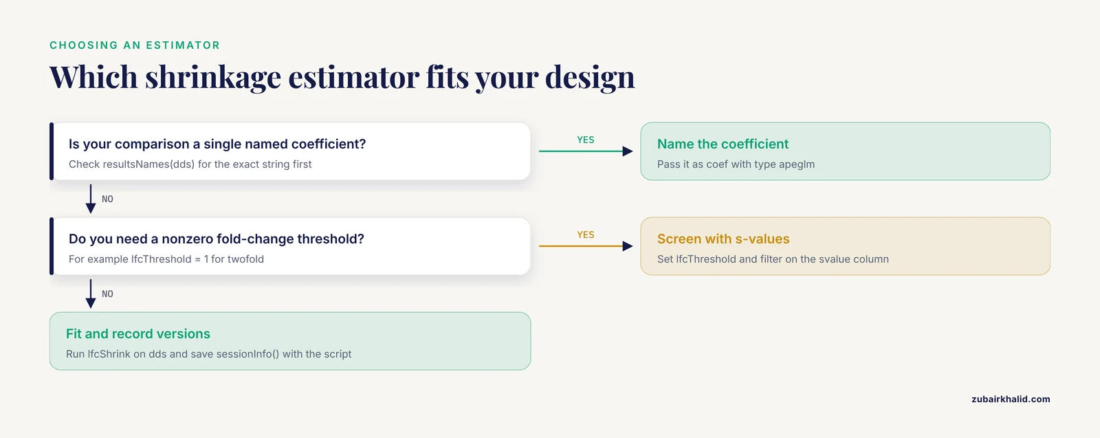
The table below is the core of the DESeq2 apeglm ashr comparison. Each row is a criterion that actually decides which estimator to type into your script.
| Feature | apeglm | ashr |
|---|---|---|
| Published method | Adaptive Student's t / Cauchy prior (Zhu, Ibrahim, and Love, Biostatistics 2018) | Adaptive shrinkage with a mixture of normal priors (Stephens, JASA 2017) |
Main lfcShrink() arguments | coef (required) | coef or contrast |
| Works with interaction contrasts | No, single coefficients only | Yes |
| Handles expanded model matrices | No | Yes |
Supports lfcThreshold screening | Yes in recent DESeq2 releases | Yes, the classic use case |
| Produces s-values | Yes when a threshold is set | Yes, especially with a threshold |
lfcSE column meaning | Posterior standard deviation | Posterior standard deviation |
| Typical relative speed | Slower as coefficient count grows | Fast per gene, scales well for single contrasts |
| Default behavior | Default type in recent DESeq2 versions | Opt-in |
| Best suited for | Standard designs with a clean coefficient name | Contrasts, interactions, threshold screening |
Both estimators return shrunken log2 fold changes and posterior standard deviations. Both preserve the base mean, p-value, and adjusted p-value columns from the standard Wald results. The differences that matter are contrast support, threshold screening, and how each handles designs with many coefficients.
Setting Up: Data, Design, and the Wald Test
Everything below assumes a standard DESeq2 workflow from a count matrix and a sample table. The full sequence, with a two-group design, looks like this.
library(DESeq2)

# cts is an integer count matrix, genes in rows, samples in columns
# coldata is a data frame with sample metadata, rownames matching colnames(cts)

dds <- DESeqDataSetFromMatrix(countData = cts,
                              colData = coldata,
                              design = ~ condition)

# Optional but recommended: drop genes with very low counts
keep <- rowSums(counts(dds)) >= 10
dds <- dds[keep, ]

dds <- DESeq(dds)
resultsNames(dds)
The resultsNames(dds) line prints the coefficient names you will pass to lfcShrink(). For a factor named condition with levels control and treated, where control is the reference, the output is "condition_treated_vs_control". Every lfcShrink() call with type = "apeglm" depends on getting this name exactly right, so make it a habit to run resultsNames(dds) before every shrinkage step.
If your reference level is not what you want, fix it before fitting.
dds$condition <- relevel(dds$condition, ref = "control")
dds <- DESeq(dds)
The main DESeq() call performs the Wald test by default. lfcShrink() operates on the fitted dds object, not on the object returned by results(). Passing a results object to lfcShrink() is one of the most frequent errors new users hit, and it appears in the troubleshooting section below.
How to Use apeglm for Shrinkage
The basic call
apeglm, short for approximate posterior estimation of generalized linear model coefficients, places an adaptive Cauchy prior on each coefficient. The prior's scale is learned from the data, and its heavy tails mean that genes with strong evidence keep their large fold changes while noisy genes get pulled hard toward zero. The method was published by Anqi Zhu, Joseph Ibrahim, and Michael Love in Biostatistics in 2018 and is distributed as its own Bioconductor package that DESeq2 calls internally.
resApe <- lfcShrink(dds,
                    coef = "condition_treated_vs_control",
                    type = "apeglm")
That is the entire operation. The returned object is a DESeqResults instance, so all downstream machinery works unchanged.
summary(resApe)
plotMA(resApe)
head(resApe[order(resApe$padj), ])
The log2FoldChange column now holds the posterior estimate, and the lfcSE column holds the posterior standard deviation rather than the Wald standard error. The MA plot after apeglm shrinkage is noticeably more linear at low mean counts, which is one of the quickest visual checks that shrinkage worked.
Key constraints of apeglm
Three constraints shape when apeglm is the right choice.
First, you must pass coef. The function will not accept contrast with type = "apeglm". If your comparison of interest is not a single coefficient in resultsNames(dds), apeglm is not the tool for that specific number.
Second, apeglm does not support expanded model matrices. Certain designs cause DESeq2 to expand the model matrix into one column per level of a factor. When that happens, lfcShrink() with apeglm stops with an error, and ashr is the documented alternative in the package vignette.
Third, apeglm's heavy-tailed prior behaves differently from a fixed normal prior at the extremes. A gene with an enormous, well-supported fold change is penalized less under a Cauchy prior than under a normal prior, because the Cauchy tails are thick. This is a feature for ranking. It keeps genuinely strong signals close to their observed values instead of over-compressing them.
apeglm with a fold-change threshold
Recent DESeq2 releases let you pass a threshold to apeglm. The estimator then computes, for each gene, the posterior probability that the true fold change lies within the threshold-bounded region, summarized as an s-value.
resApeT <- lfcShrink(dds,
                     coef = "condition_treated_vs_control",
                     type = "apeglm",
                     lfcThreshold = 1)
An s-value is the local false sign rate for the interval you specified. It answers a different question than a p-value. Instead of asking whether the effect differs from zero, it bounds the posterior probability that the true effect falls inside the uninteresting region. When a nonzero lfcThreshold is set, the returned object drops the p-value and adjusted p-value columns and reports the s-value instead. Plan your downstream filtering around that change.
How to Use ashr for Shrinkage
The basic call
ashr, short for adaptive shrinkage, was published by Matthew Stephens in the Journal of the American Statistical Association in 2017. It models each effect size as drawn from a mixture of normal distributions at different scales, including a point mass at zero, and estimates the mixture weights from all genes simultaneously. The posterior estimate per gene reflects how much the data as a whole look like they contain many null effects and a few large ones.
resAsh <- lfcShrink(dds,
                    contrast = c("condition", "treated", "control"),
                    type = "ashr")
Note the flexibility. type = "ashr" accepts either coef or contrast. The contrast argument takes the same three-element vector form used in results(), naming the factor, the numerator level, and the denominator level. This single property resolves the main limitation of apeglm.
Contrasts and interaction terms
The clearest advantage of ashr shows up in designs with interactions. Consider a design of ~ genotype + condition + genotype:condition. The interaction coefficient tests whether the treatment effect differs between genotypes, but it is expressed on the interaction scale and is awkward to name as a single coef. With ashr you can shrink an arbitrary contrast directly.
resInt <- lfcShrink(dds,
                    contrast = list("genotypeMutant.conditionTreated"),
                    type = "ashr")
The same flexibility applies to contrasts across multiple model terms, such as comparing a combined condition and time point against another combination in a time-course experiment. For any of these, the vignette for DESeq2 recommends ashr.
Threshold screening with s-values
The second major use of ashr is threshold-based screening. Many projects do not care about genes with tiny fold changes, even if those changes are statistically solid with 40 million reads per sample. Screening on adjusted p-value alone promotes thousands of genes with 1.05-fold changes that no assay can validate.
resAshT <- lfcShrink(dds,
                     coef = "condition_treated_vs_control",
                     type = "ashr",
                     lfcThreshold = 1)
With lfcThreshold = 1, you test against a twofold change rather than a change of exactly 1. The returned object replaces p-value and adjusted p-value columns with an s-value. Sort by s-value and filter at a cutoff such as 0.05 to get a list of genes whose true fold change is likely outside the threshold region.
Practical notes for ashr
The lfcSE column again holds the posterior standard deviation. ashr also exposes a svalue column even without a threshold in current DESeq2 output, which you can use as an additional ranking statistic alongside padj. The estimator fits an expectation maximization procedure per gene, and runtime scales comfortably for typical gene counts on a single core, with BiocParallel support if you enable parallel = TRUE.
The DESeq2 apeglm and ashr Comparison in Detail
Readers searching for the best deseq2 apeglm ashr comparison usually want one thing answered: which one should I use for my experiment. The honest answer is that for a simple two-group design, either produces nearly identical results, and the choice is about workflow convenience. For complex designs, the answer is firmer. Here is how the comparison options break down criterion by criterion.
Shrinkage behavior and prior shape
Both estimators are adaptive, meaning the amount of shrinkage depends on the data rather than on a fixed setting. Both shrink noisy, low-count genes strongly and leave well-supported effects nearly intact. The distinction lies in prior geometry. apeglm uses a single heavy-tailed prior whose scale adapts to the data, while ashr uses a discrete mixture of normal priors whose weights adapt per gene. In practice, for two-group designs, the shrunken fold changes from the two methods correlate extremely closely, and the ranking of top genes is usually stable across methods. If a top hit appears under one estimator and vanishes under the other, that gene sits in the ambiguous middle range where posterior support is genuinely borderline, and you should treat it with suspicion regardless of method.
Contrast support
This is the sharpest difference. apeglm requires a single named coefficient. ashr accepts contrasts. Concretely:
# Works with apeglm
resultsNames(dds)  # "condition_treated_vs_control"
resApe <- lfcShrink(dds, coef = "condition_treated_vs_control", type = "apeglm")

# Works only with ashr among the two recommended types
resAsh <- lfcShrink(dds, contrast = c("condition", "treated", "control"), type = "ashr")
If your design uses ~ batch + condition and you want the condition effect adjusted for batch, both work, because condition_treated_vs_control remains a single coefficient. If your design uses interactions, paired structures, or group-level comparisons where the quantity of interest is a difference of coefficients, ashr is the correct tool.
Threshold screening and s-values
When you filter on padj alone, you test against a null of exactly zero fold change. The lfcThreshold workflow tests against a region of biological indifference instead. The pros and cons of threshold screening deserve their own framing.
Pros: the resulting gene list maps directly onto validation experiments, because every reported gene clears a fold-change bar you chose in advance. Cons: you lose conventional p-value output and must explain s-values to collaborators, and the threshold you pick is a biological judgment, not a statistical default. A threshold of 1 on the log2 scale means twofold. A threshold of 0.585 corresponds to a 1.5-fold change. Choose it before looking at the data, the same way you would choose an alpha level.
Speed, scale, and reproducibility
apeglm's runtime grows with the number of coefficients in the design. A 12-sample two-group experiment shrinks in seconds. A 200-sample design with batch, cell type, and interaction terms takes longer, and the cost repeats if you shrink several coefficients. ashr fits efficiently per gene and handles multi-coefficient designs well. Both support parallel evaluation.
resApe <- lfcShrink(dds,
                    coef = "condition_treated_vs_control",
                    type = "apeglm",
                    parallel = TRUE,
                    BPPARAM = BiocParallel::MulticoreParam(4))
For reproducibility, record the DESeq2, apeglm, and ashr package versions with sessionInfo() in every analysis. Shrinkage estimates are deterministic given the data and versions, so version drift is the main reproducibility risk.
The pros and cons summary
apeglm pros: it is the DESeq2 default in recent versions, it produces excellent rankings for standard designs, its heavy-tailed prior preserves strong signals, and its output slots directly into every DESeqResults workflow.
apeglm cons: it requires coef, it rejects contrasts, it fails on expanded model matrices, and runtime grows with design complexity.
ashr pros: it supports both coef and contrast, it handles interaction terms and expanded matrices, it powers the lfcThreshold and s-value workflow, and it scales well.
ashr cons: it is opt-in rather than default, s-value output requires explanation in methods sections, and the mixture fitting adds a per-gene computational step.
Neither estimator is wrong for a two-group comparison. The deseq2 apeglm ashr comparison resolves into a design question, not a quality question.
Worked Scenarios
Scenario 1: Two-group comparison, ranking for validation
A researcher has 6 control and 6 treated samples, a design of ~ condition, and wants a ranked list of genes for qPCR validation. The full shrinkage workflow is short.
dds <- DESeqDataSetFromMatrix(cts, coldata, design = ~ condition)
dds$condition <- relevel(dds$condition, ref = "control")
dds <- dds[rowSums(counts(dds)) >= 10, ]
dds <- DESeq(dds)
resApe <- lfcShrink(dds, coef = "condition_treated_vs_control", type = "apeglm")
resApeOrd <- resApe[order(resApe$padj, -abs(resApe$log2FoldChange)), ]
head(resApeOrd, 20)
Ranking on adjusted p-value first and shrunken effect size second gives genes that are both statistically solid and biologically sizeable. Take the top 20 for primer design. apeglm is a natural fit here because the comparison is a single coefficient and the heavy-tailed prior ranks strong responders honestly.
Scenario 2: Interaction design
A researcher compares two genotypes under two treatments with the design ~ genotype + treatment + genotype:treatment. The interest lies in genes whose treatment response differs by genotype.
dds <- DESeqDataSetFromMatrix(cts, coldata, design = ~ genotype + treatment + genotype:treatment)
dds <- DESeq(dds)
resultsNames(dds)
The main effects can be shrunk with apeglm by coefficient. The interaction, however, is best handled with ashr using a contrast or a list-based contrast.
resMain <- lfcShrink(dds, coef = "genotype_Mutant_vs_WT", type = "apeglm")
resInt  <- lfcShrink(dds, contrast = list("genotypeMutant.treatmentTreated"), type = "ashr")
Using ashr for the interaction, or simply using ashr for every shrinkage step in this project, avoids the constraint that apeglm places on coefficient selection.
Scenario 3: Screening for twofold changes across many genes
A screening team wants genes with at least a twofold change, ranked by confidence in that statement.
resScr <- lfcShrink(dds,
                    coef = "condition_treated_vs_control",
                    type = "ashr",
                    lfcThreshold = 1)
resScr[order(resScr$svalue), ]
sig <- subset(as.data.frame(resScr), svalue < 0.05)
nrow(sig)
The s-value column supports the claim each reviewer will ask about: how likely is it that this gene's true effect is actually below twofold. Running the same call with type = "apeglm" gives a comparable thresholded ranking in recent DESeq2 versions, so the s-value workflow is not locked to ashr. The classic and best-documented route, though, is ashr.
Practical Details That Affect Interpretation
Three details catch analysts who are new to lfcShrink() output.
The stat column changes meaning. After apeglm or ashr shrinkage, the statistic is computed from the shrunken effect and its posterior standard deviation. The p-value and adjusted p-value columns, however, still come from the original Wald test on the unshrunken fit. Do not compute a new p-value from the shrunken statistic and expect it to match, and do not present the shrunken statistic as the test statistic in a methods section without explanation.
Shrinkage is for reporting effect sizes and ranking. The standard significance calls come from results(dds). Many analysts keep both objects, one for significance and one for effect sizes, and merge them by gene identifier.
resRaw <- results(dds)
resShr <- lfcShrink(dds, coef = "condition_treated_vs_control", type = "apeglm")
merged <- data.frame(resRaw, lfcShrunk = resShr$log2FoldChange)
Volcano plots drawn from shrunken fold changes look cleaner at the extremes because the low-count funnel is gone, but the p-values on the y-axis remain the unshrunken Wald p-values. Label your axis as shrunken log2 fold change to keep the figure honest.
Troubleshooting Common Errors
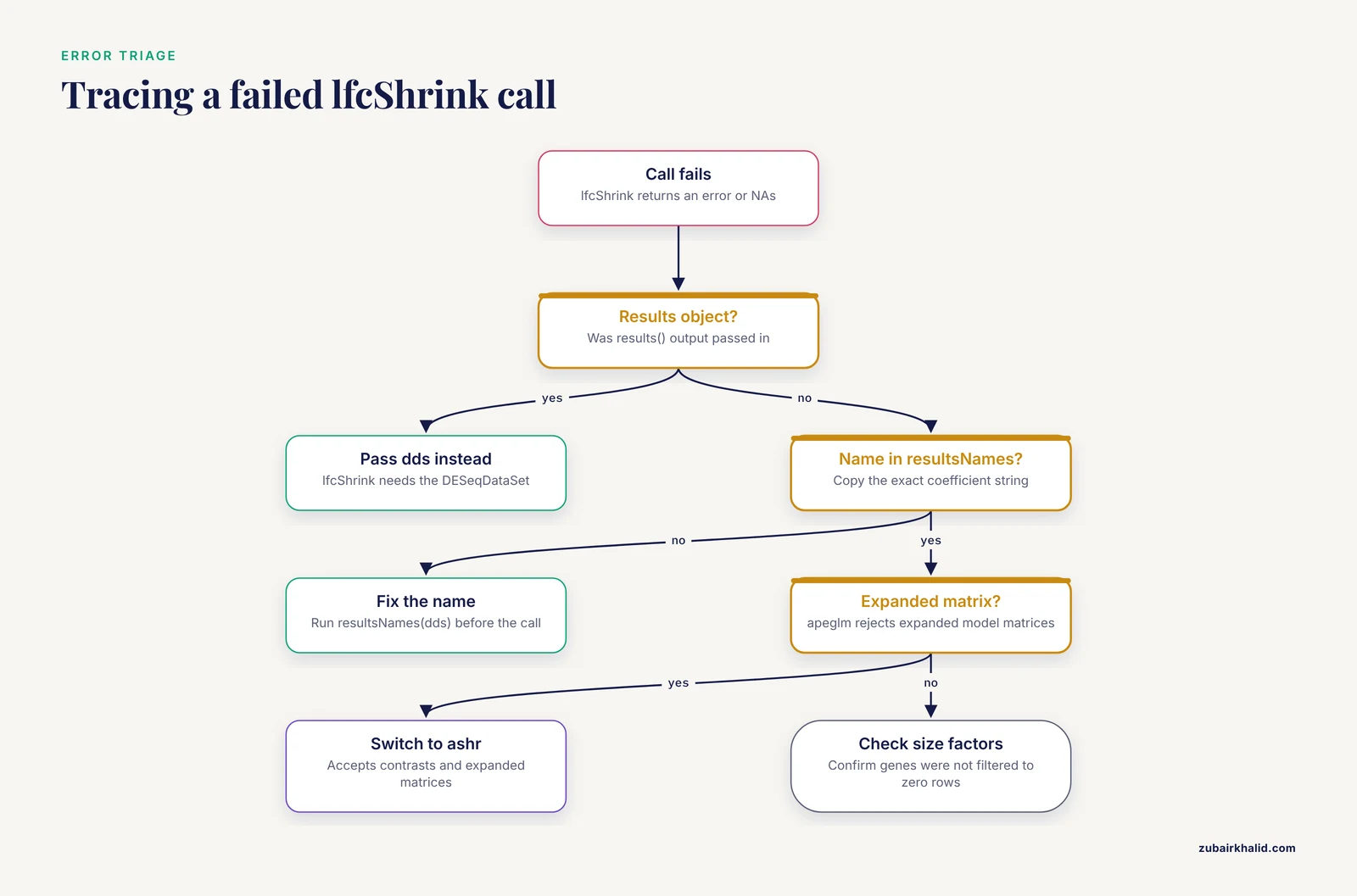
RNA-seq analysis generates a predictable set of error messages around shrinkage. Each entry below gives the symptom, the cause, and the fix. This section addresses the rna seq error patterns that account for most stalls in real projects.
apeglm demands a coefficient
Symptom: an error stating that the coefficient must be specified, or that type = "apeglm" cannot be used with contrast.
Cause: apeglm supports only named coefficients.
Fix: use coef with a name from resultsNames(dds), or switch to type = "ashr" for that call.
The coefficient name is wrong
Symptom: an error that the given coefficient is not among the model coefficient names.
Cause: a typo, or the reference level changed after fitting, which changes coefficient names.
Fix: run resultsNames(dds) immediately before lfcShrink() and copy the exact string. Use relevel() before DESeq() if the reference level is wrong.
Passing a results object instead of the dataset
Symptom: an error when calling lfcShrink() on the object returned by results().
Cause: lfcShrink() operates on the DESeqDataSet, because it needs the model information to refit coefficients.
Fix: always call lfcShrink(dds, ...) and keep the results() output as a separate object.
Every gene gets NA for fold change
Symptom: log2FoldChange is NA for most or all genes in the shrunken results.
Cause: most often, the count matrix was filtered to zero rows, or the size factors are invalid. A related upstream error is a message that every gene contains at least one zero and log geometric means cannot be computed, which blocks size factor estimation.
Fix: check summary(dds) and sizeFactors(dds). For sparse single-cell-style matrices or metagenomic count tables, estimate size factors with the geometric mean control features or supply size factors directly. Confirm that genes were not filtered out by an over-aggressive prefilter.
A subset of genes has NA fold changes
Symptom: a small fraction of rows shows NA for fold change and standard error.
Cause: automatic outlier replacement flagged genes by Cook's distance when the number of replicates is small, or genes have all zero counts in one group.
Fix: these genes are excluded from testing by design when the replacement is not possible. Report the count of affected genes. With more replicates, more genes become testable.
Adjusted p-values are NA for many genes
Symptom: padj is NA for a large block of genes with valid p-values.
Cause: independent filtering. DESeq2 excludes genes whose mean normalized count is too low for the multiple testing procedure to ever reach significance, which conserves power for the testable set.
Fix: this is expected behavior, not an error. Inspect the filter threshold with metadata(res)$filterThreshold if you need to document it.
Shrinkage takes too long
Symptom: lfcShrink() with apeglm runs for hours on a large design.
Cause: apeglm cost scales with the number of coefficients. Designs with many factor levels and interactions generate many columns.
Fix: enable parallel evaluation with parallel = TRUE and a BiocParallel backend, shrink only the coefficients you will report, or switch to ashr for the slow calls.
Results differ between collaborators
Symptom: two analysts report different shrunken fold changes for the same data.
Cause: different DESeq2 versions, different reference levels, or one analyst shrinking after results() with a different factor ordering.
Fix: compare sessionInfo() output, align reference levels with relevel(), and share the exact lfcShrink() call in the analysis script.
General bioinformatics troubleshooting advice applies here in a specific form. Save intermediate objects with saveRDS() so that a failed shrinkage call does not force a refit of the entire pipeline. Print resultsNames(dds) into your log files. Keep one script that runs from raw counts to shrunken results without manual steps in between, because manual environment state is the most common source of irreproducible RNA-seq numbers.
Common Mistakes and Limitations
The mistakes below appear repeatedly in review comments and on support forums. Each is avoidable with one deliberate step.
Calling lfcShrink() on a results object instead of the dds object. The shrinkage function refits coefficients against the dataset, so it needs the dataset.
Filtering on shrunken fold change and unshrunken adjusted p-value inconsistently across figures. Decide once, per project, which object feeds each figure, and note the choice in your methods.
Presenting lfcSE after shrinkage as the Wald standard error. For apeglm and ashr, that column is a posterior standard deviation. The distinction matters when readers compare your reported uncertainty to raw results() output.
Using a shrunken effect size to claim significance. Significance comes from the Wald test. Shrunken effect sizes describe magnitude, not evidence.
Interpreting an s-value as a p-value. An s-value bounds the posterior probability that the true effect lies in the region you declared uninteresting. It answers a question about effect size, not a question about the null hypothesis of zero effect.
Choosing a fold-change threshold after seeing the results. Set lfcThreshold from experimental reasoning, such as the detection floor of your validation platform, before ranking genes.
Ignoring reference levels. A reversed contrast flips every sign in your tables and figures, and the numbers remain internally consistent, so the error propagates quietly through an entire manuscript.
Regarding limitations, individual projects vary in design, depth, and biological noise, and any single set of default choices cannot cover every analysis. Consult the DESeq2 vignette for your installed version, because interface details such as default shrinkage type and threshold support have evolved across releases. For design decisions specific to your experiment, a consulting session with a statistical geneticist is worth the time.
Frequently Asked Questions
Does lfcShrink change my p-values?
No. P-values and adjusted p-values come from the original Wald test on the unshrunken coefficients. Shrinkage replaces the fold-change estimate and its standard error, and the p-value columns carry over unchanged unless you set a nonzero lfcThreshold, in which case they are replaced by an s-value.
Can I use apeglm with a contrast instead of a coefficient?
No. apeglm in DESeq2 requires the coef argument with a name from resultsNames(dds). For any comparison that is not a single coefficient, including interaction contrasts, use type = "ashr".
Which estimator should I use for an interaction term?
Use ashr. It accepts contrast specifications and expanded model matrices, so it can shrink the specific difference of coefficients you care about, while apeglm is limited to single named coefficients.
What is an s-value and when does it replace padj?
An s-value is a local false sign rate for a threshold-bounded region, meaning it bounds the posterior probability that the true fold change falls inside the region you declared uninteresting. It replaces the p-value and adjusted p-value columns when you pass a nonzero lfcThreshold to lfcShrink().
Do apeglm and ashr give different answers for a simple two-group comparison?
For a clean two-group design the shrunken fold changes from the two methods are nearly identical, and top gene rankings are usually stable. The estimators differ mainly in contrast support, threshold screening, and behavior on complex designs, not in basic two-group output.
Should I still use the normal shrinkage type?
No, not for new analyses. The type = "normal" estimator remains available for backward compatibility with older scripts and its historical results, but the DESeq2 documentation recommends apeglm or ashr for current work, and recent package versions default to apeglm.