Using Bioconductor DelayedArray for Large Genomic Data in R
By Dr. Zubair Khalid, DVM, MS, PhD ·

After working through this guide you will be able to take a gene by sample or gene by cell matrix that is several times larger than your RAM, store it in an HDF5 file, subset it, compute row and column statistics across it in parallel, save it inside a SummarizedExperiment, and hand it to downstream Bioconductor packages without ever loading the full dataset into memory. Those are the practical skills behind out-of-memory analysis in R for bioinformatics, and the DelayedArray package from the Bioconductor project provides them.
You will need:
- A recent R release (4.4 or newer) with Bioconductor installed through BiocManager.
- About 8 GB of RAM. Every example in this Bioconductor tutorial runs on a laptop.
- Data on a local disk rather than a network share, because HDF5 read speed depends on disk latency.
- For the single-cell section, a Cell Ranger filtered_feature_bc_matrix.h5 file if you have one. Every other example generates its own data.
Why Ordinary R Objects Run Out of Memory on Large Genomic Data
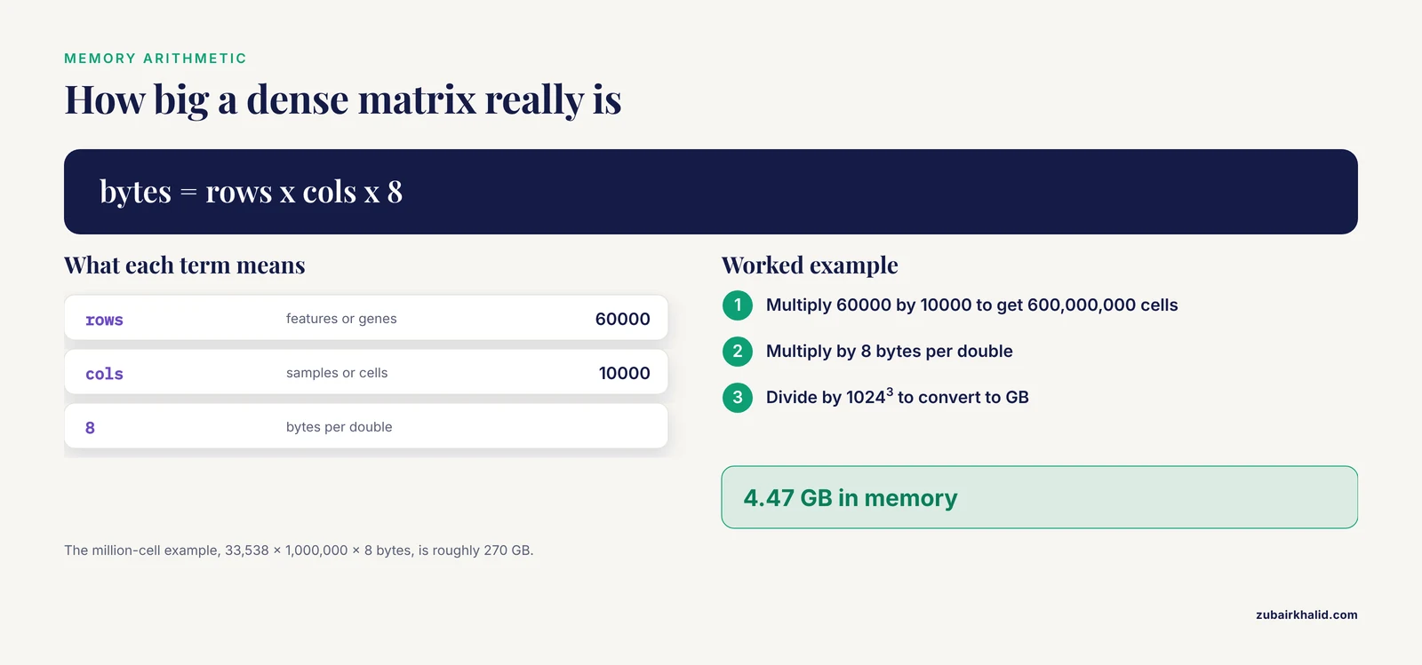
R keeps every object in RAM, and the arithmetic is unforgiving. A dense double-precision matrix of 60,000 features by 10,000 samples occupies 60,000 x 10,000 x 8 bytes, about 4.5 GB. A million-cell single-cell dataset with 33,538 genes occupies 33,538 x 1,000,000 x 8 bytes, roughly 270 GB, before any copies. R also copies data during many transformations, so peak usage often reaches two to three times the size of the object you thought you had.
This limitation is not hypothetical. The BESSiE authors state it plainly in their rationale for moving large-scale genomic marker analysis out of R, noting that script based environments like R may not be able to handle large-scale genomic data or exploit model properties that save computing time and memory [1]. The PRSice-2 developers hit the same wall at biobank scale and rebuilt their polygenic risk score software specifically to be dramatically faster and more memory-efficient than earlier tools [2].
The Bioconductor answer is out-of-memory representation. The curatedTCGAData and cBioPortalData packages serve large methylation datasets through out-of-memory data representation so that loading stays responsive and analysis remains possible on machines with limited memory [3]. The recount3 resource applies the same philosophy at repository scale, offering summaries and queries over more than 750,000 uniformly processed human and mouse RNA-seq samples through R and Bioconductor packages instead of raw downloads [4]. DelayedArray is the machinery underneath both.
How DelayedArray Works: Seeds, Delayed Operations, and Realization
Three ideas carry the whole package.
A seed is any array-like object that can report its dimensions, dimnames, and data type, and can return a requested subarray on demand. Seeds include ordinary matrices, sparse dgCMatrix objects from the Matrix package, dense HDF5 datasets on disk, and sparse HDF5 datasets of the kind Cell Ranger writes.
Delayed operations build a recipe instead of computing. When you write log1p(da + 1) on a DelayedArray, R records that recipe. Nothing touches the data until a concrete value is required.
Realization executes the recipe in blocks. When you call as.matrix, colSums, or writeHDF5Array, DelayedArray walks the data in tiles that fit in RAM, applies the operation tile by tile, and assembles the result. Two size knobs control this. The chunk is the on-disk storage unit of an HDF5 dataset. The block is the in-memory working tile used during processing. Blocks are assembled from chunks. Keep chunks in the low megabytes and set the block size to a large fraction of your free RAM.
In day-to-day coding the behavior sorts into three groups:
- Operations that stay delayed and cost almost nothing: subsetting, t(), cbind(), rbind(), arithmetic, log() and other transformations, comparisons, and is.na().
- Operations that stream in blocks and return a small result: colSums(), rowMeans(), sum(), max(), and the DelayedMatrixStats equivalents.
- Operations that force full realization into memory: as.matrix(), as.array(), as.vector(), as.data.frame(), and which().
This design is why SummarizedExperiment assays, SingleCellExperiment objects, and MultiAssayExperiment containers can hold data far larger than RAM [3]. It is also why new infrastructure keeps appearing on the same foundation, for example DeeDeeExperiment, which extends SingleCellExperiment to manage large collections of differential expression and enrichment results [5], and BiocMAP, a Bioconductor-friendly bisulfite sequencing pipeline built around memory-efficient representation of WGBS output [6].
Step-by-Step: DelayedArray for Large Genomic Data
The walkthrough below builds from a toy matrix to patterns that scale. Run each block in order.
Step 1. Install and Load the Packages
if (!requireNamespace("BiocManager", quietly = TRUE))
    install.packages("BiocManager")

BiocManager::install(c(
  "DelayedArray", "HDF5Array", "DelayedMatrixStats", "rhdf5",
  "SummarizedExperiment", "SingleCellExperiment",
  "BiocParallel", "Matrix",
  "scran", "scater"   # optional, used in the single-cell step
))
Then attach what the early steps need:
library(DelayedArray)
library(HDF5Array)
library(DelayedMatrixStats)
library(rhdf5)
DelayedArray provides the delayed evaluation framework. HDF5Array provides the on-disk seeds, the writer, the readers for 10x and sparse HDF5 files, and the SummarizedExperiment savers. If you call writeHDF5Array without attaching HDF5Array you will see Error: could not find function "writeHDF5Array", and the fix is simply library(HDF5Array).
Step 2. Wrap an In-Memory Matrix and Inspect It
set.seed(1)
counts <- matrix(rpois(12, lambda = 5), nrow = 4)
dimnames(counts) <- list(
  gene   = paste0("GENE", 1:4),
  sample = paste0("S", 1:3)
)

da <- DelayedArray(counts)
da
Expected output (values are illustrative, the header line is what to look for):
<4 x 3> matrix of class DelayedMatrix and type "integer":
       S1 S2 S3
GENE1   4  3  6
GENE2   5  6  4
GENE3   3  7  5
GENE4   6  4  3
class(da) # a DelayedMatrix, the 2-dimensional DelayedArray
type(da) # "integer"
seed(da) # the wrapped matrix, the thing operations run against
d2 <- log1p(da + 1) # recorded, not computed
d2 # still a DelayedMatrix
m <- as.matrix(d2) # realization happens here, returns an ordinary matrixPrinting a DelayedArray is always safe because the show method prints only a preview, even for a terabyte-scale object. Also note the type. Integer counts occupy half the disk space of doubles, and DelayedArray preserves the type of its input, so check type() before and after writing.
Step 3. Write the Data to HDF5 with Sensible Chunks
h5_counts <- writeHDF5Array(
  da,
  filepath = "counts_small.h5",
  name     = "counts",
  chunkdim = c(4, 1),
  level    = 6
)
# writing the same dataset name twice into one file errors,
# use a fresh file or name when rerunning

h5_counts
# <4 x 3> matrix of class HDF5Array and type "integer"

file.size("counts_small.h5")   # a few kilobytes for this toy example

rhdf5::h5ls("counts_small.h5")
name group otype dclass dim
1 counts / H5I_DATASET INTEGER 4 x 3Two parameters matter here.
chunkdim sets the shape of each on-disk chunk. c(4, 1) stores one sample per chunk, which makes column-wise operations such as per-sample sums read contiguous data. If your dominant operation is per-gene, use c(1, ncol) instead. If you leave chunkdim out, HDF5Array picks chunk dimensions automatically with small chunks as the goal.
level sets the gzip compression level from 0 to 9. Level 6 is a balanced choice. Level 0 writes faster and larger. Count matrices compress well, often several-fold.
Scale check for a realistic bulk dataset:
# 60,000 features x 10,000 samples as doubles
60000 * 10000 * 8 / 1024^3
# 4.47 GB in memory

# a chunk of c(1000, 500) doubles
1000 * 500 * 8 / 1024^2
# 3.81 MB per chunk, a good size to keep reads efficient
Step 4. Read Back, Subset, and Compute Without Loading Everything
counts_h5 <- HDF5Array("counts_small.h5", "counts")

# writeHDF5Array does not store row and column names, attach them once
h5writeDimnames(dimnames(counts), "counts_small.h5", "counts")

counts_h5 <- HDF5Array("counts_small.h5", "counts")
dimnames(counts_h5)   # now matches the original

counts_h5[1:2, 2:3]   # reads only the chunks that contain these values
colSums(counts_h5)    # streams through all chunks, returns a numeric vector
chunkdim(counts_h5)   # c(4, 1)
is_sparse(counts_h5)  # FALSE for this dense dataset
HDF5Array() opens the file lazily and read-only, so constructing the object is instant no matter how large the file is. Subsetting is delayed and cheap. The cost appears only when a result is realized, and then it is proportional to the chunks touched, not to the size of the file.
Step 5. Control Block Size and Run Block-Wise Parallel Code
library(BiocParallel)

getAutoBlockSize()
# 12582912, the 12 MB default, conservative for simple streaming statistics

setAutoBlockSize(512 * 1024^2)   # 512 MB blocks

# one-liner statistics, block-processed for you
DelayedMatrixStats::colMeans2(counts_h5)
DelayedMatrixStats::rowVars(counts_h5)

# custom block-wise code with a parallel backend
res <- blockApply(
  counts_h5,
  function(block) colMeans(block),
  grid    = colAutoGrid(counts_h5),
  BPPARAM = MulticoreParam(workers = 4)
)
unlist(res)
colAutoGrid() builds blocks that span all rows and a run of columns sized to fit the block size. With 512 MB blocks and 8-byte doubles, each block holds about 67 million elements. Memory during a parallel run is roughly block size times workers, so 4 workers at 512 MB means about 2 GB plus copies. Set the block size with that multiplication in mind.
Use DelayedMatrixStats when a function already exists for your statistic, for example rowVars(), colMeans2(), or colQuantiles(). Reach for blockApply() when you need something custom, such as a per-column trimmed mean or a two-pass statistic.
Step 6. Work with Sparse Single-Cell Matrices
Single-cell count matrices are mostly zeros, and storage and arithmetic should exploit that.
# any Cell Ranger filtered_feature_bc_matrix.h5
mat <- TENxMatrix("filtered_feature_bc_matrix.h5", group = "matrix")
is_sparse(mat)     # TRUE
sparsity(mat)      # around 0.9 for a typical peripheral blood mononuclear cell sample
The savings are large. For a 33,538 gene by 2,700 cell matrix:
33538 * 2700 * 8 / 1024^2
# 691 MB as a dense double matrix

# at 5 percent nonzero entries, CSC sparse storage needs about
33538 * 2700 * 0.05 * 12 / 1024^2
# 52 MB, one value and one integer index per nonzero element
TENxMatrix() reads the 10x Genomics HDF5 layout. H5SparseMatrix() reads any HDF5 sparse CSC dataset, and DelayedArray() also wraps in-memory dgCMatrix objects directly:
set.seed(2)
sparse_counts <- Matrix::Matrix(
  rpois(200000, lambda = 0.05), nrow = 1000, sparse = TRUE
)
is_sparse(DelayedArray(sparse_counts))   # TRUE, an in-memory sparse seed
Downstream single-cell packages read these backends block by block:
library(SingleCellExperiment)
sce <- SingleCellExperiment(assays = list(counts = mat))
sce <- scran::computeSumFactors(sce)
sce <- scater::logNormCounts(sce)
scran and scater use the beachmat C++ layer, which reads DelayedMatrix backends in blocks, so these calls never load the full counts matrix into RAM.
Step 7. Put a SummarizedExperiment on Disk
library(SummarizedExperiment)

se <- SummarizedExperiment(
  assays  = list(counts = counts_h5),
  colData = DataFrame(treatment = factor(c("ctrl", "ctrl", "treated")))
)

saveHDF5SummarizedExperiment(se, dir = "se_h5", as.sparse = TRUE)
# the call errors if se_h5 already exists, remove it first

se2 <- loadHDF5SummarizedExperiment("se_h5")
assay(se2, "counts")   # an HDF5Array again, data stays on disk
as.sparse = TRUE stores count-like assays as a sparse HDF5 dataset. The directory holds the HDF5 file plus the serialized row and column data, and loadHDF5SummarizedExperiment() rebuilds the full object. This is the storage pattern that large Bioconductor data resources use for out-of-memory methylation and multiomics containers [3], and it is the foundation that newer classes such as DeeDeeExperiment build on [5]. Give a relative dir when you plan to move the object, because the serialized parts remember the path you provided.
Step 8. Realize Results Deliberately
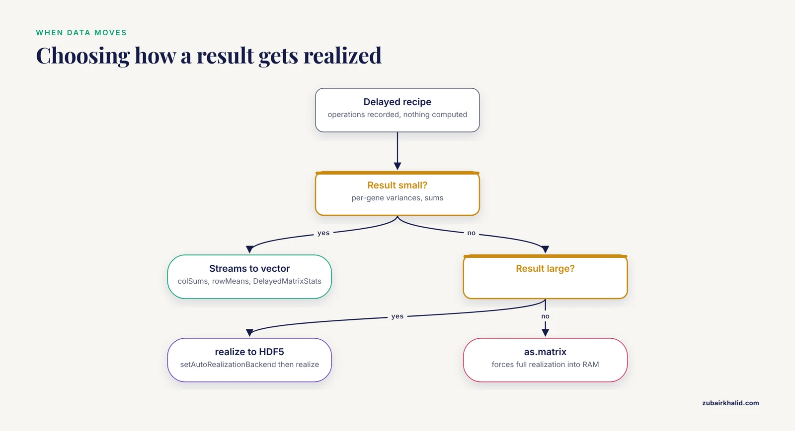
Some results are small and belong in memory, such as per-gene variances. Others are large and belong on disk.
setAutoRealizationBackend(HDF5ArrayRealizationBackend())
scaled <- realize(log1p(counts_h5 + 1))   # written to disk, not RAM
class(scaled)                             # a DelayedMatrix backed by the dump file
getHDF5DumpFile()                         # where the result went

setAutoRealizationBackend(NULL)           # back to the in-memory default
By default the realization dump goes to the R session temporary directory, which getHDF5DumpDir() shows, so auto-realized intermediates disappear when the session ends. Call setHDF5DumpFile() to point the dump at a file you choose, or use writeHDF5Array() when you want full control of the path and dataset name.
Step 9. Verify the Result Is Right
Delayed pipelines fail quietly when a chunk is read with the wrong shape or a dimname is lost, so check against the in-memory original whenever possible.
counts_h5 <- HDF5Array("counts_small.h5", "counts")

stopifnot(identical(dim(counts), dim(counts_h5)))
stopifnot(identical(dimnames(counts), dimnames(counts_h5)))
stopifnot(all.equal(as.matrix(counts_h5), counts))
stopifnot(all.equal(colSums(counts_h5), colSums(counts)))
stopifnot(all.equal(
  DelayedMatrixStats::colMeans2(counts_h5),
  colMeans(counts)
))
For larger files, spot check a random subset and inspect the file structure:
i <- sample(nrow(counts_h5), 2)
j <- sample(ncol(counts_h5), 1)
stopifnot(all.equal(
  as.matrix(counts_h5[i, j, drop = FALSE]),
  counts[i, j, drop = FALSE]
))

rhdf5::h5ls("counts_small.h5")   # dataset names, storage classes, dimensions
If every check passes, the on-disk object is a faithful copy of the original.
Key Options at a Glance
| Function or argument | What it controls | Practical choice |
|---|---|---|
| , - | , - | , - |
| writeHDF5Array(chunkdim) | Shape of on-disk HDF5 chunks | c(1000, 500) for a 60,000 x 10,000 gene by sample matrix |
| writeHDF5Array(level) | Gzip compression level, 0 to 9 | 6 for a balance of size and speed, 0 for fastest writes |
| setAutoBlockSize(n) | RAM used per block during block processing | 512 MB to 2 GB, divided across workers |
| setAutoRealizationBackend() | Where realize() writes results | HDF5ArrayRealizationBackend() for persistent intermediates |
| blockApply(grid, BPPARAM) | Custom block-wise code and parallel backend | colAutoGrid(x) with MulticoreParam(workers = 4) |
| TENxMatrix(group) | Reader for 10x Genomics HDF5 files | group = "matrix" |
| saveHDF5SummarizedExperiment(as.sparse) | Sparse on-disk storage for count assays | as.sparse = TRUE for count-like data |
| h5writeDimnames() | Attaches row and column names to an HDF5 dataset | Call right after writeHDF5Array |
| DelayedMatrixStats functions | Block-wise matrix statistics | Use instead of matrixStats on DelayedMatrix |
Practical Tips for Speed and Memory
- Decide the dominant access pattern before you write. Column-wise statistics want chunks that span rows in tall thin blocks, gene-wise statistics want the opposite. Changing the on-disk layout later means rewriting the file.
- Raise the block size for streaming statistics. The 12 MB default is safe but slow for simple passes over a large file. A 512 MB to 2 GB block turns most jobs into a handful of sequential reads. Remember the formula, block elements times 8 bytes for doubles.
- Sort subscript indices before subsetting. counts_h5[sort(i), ] touches chunks in order and then you reorder the small result. Random index order turns one sequential read into thousands of scattered chunk reads.
- Realize reused intermediates once. If a normalized or scaled matrix feeds five downstream steps, realize it to HDF5 under a clear name and reuse the file. Repeating the same delayed recipe in a loop recomputes every block every time.
- Prefer DelayedMatrixStats over apply(). apply(x, 1, mean) on a DelayedMatrix walks the data in an awkward direction and pays R function call overhead per unit. rowMeans() or DelayedMatrixStats::rowMeans2() streams the same computation in optimized blocks.
- Query before you download. Resources built on this infrastructure let you pull only what you need. recount3 supports queries for specific genes, junctions, and samples rather than whole-study downloads [4], and OmicsMLRepoR supports repository-wide queries over harmonized metadata from hundreds of thousands of samples [7].
- Check sparsity() before choosing a backend. If most values are zero, a sparse seed saves an order of magnitude in space and IO. Compressed representations are the norm in large-scale methylation tooling, for example NanoMethViz manages large nanopore methylation datasets with a compressed data format [8].
- Pick normalization code that respects the backend. CONSTANd provides normalization in R and Bioconductor designed for both small and large scale omics experiments, which fits pipelines where the count matrix never sits in RAM [9].
- Keep data local and watch the temp directory. Auto-realized intermediates land in tempdir() by default and vanish with the session. A large realize() call can also fill a small disk, so check free space before realizing a multi-gigabyte result.
- Match tools to scale. Even within Bioconductor, some methods were slow for large inputs and were rebuilt for it, which is the motivation behind matchRanges for efficient generation of matched null genomic ranges [10]. When a workflow feels slow, look for a block-aware implementation before writing your own.
Common Mistakes and Limitations
Accidental realization. The most expensive error is calling a realizing function on a huge object. which(mat > 0) builds a full logical mask in memory before returning indices. For the 2,700-cell example that mask is about 362 MB, and at a million cells it is about 134 GB, at which point R answers with Error: cannot allocate vector of size 124.9 Gb or simply kills the session. Count zeros per column with DelayedMatrixStats::colCounts(mat, value = 0) instead, or fold the logic into blockApply(). The same trap hides inside as.data.frame(), as.vector(), and any modeling function that calls as.matrix() internally.
Block size multiplied by workers. setAutoBlockSize(2 * 1024^3) with MulticoreParam(workers = 8) can request 16 GB or more once copies are counted. Set the block size to roughly free RAM divided by worker count, with a safety factor of two.
Chunk shape that fights your access pattern. Chunks of c(1, ncol) make every per-sample summary touch tens of thousands of tiny chunks. If you already inherited a badly shaped file, a delayed t() is free, but realizing the transpose writes a new file, so budget the time and disk once rather than paying on every analysis.
Dimnames that vanish at the write step. writeHDF5Array() stores values, not names. Without h5writeDimnames(), a reloaded matrix has NULL dimnames and downstream code that indexes by gene symbol breaks with a subscript out of bounds error. Write the dimnames and verify with dimnames() after reloading.
Broken file paths after moving data. An RDS containing an HDF5Array stores the path to the file. Move the RDS without the HDF5 file and the next read fails with an error mentioning H5Fopen or an inability to open the file. Ship the HDF5 file together with the RDS, prefer relative paths, and use the saveHDF5SummarizedExperiment() and loadHDF5SummarizedExperiment() pair for whole objects.
matrixStats called on a DelayedMatrix. The original matrixStats functions expect in-memory matrices and coerce, which is exactly the memory spike you were avoiding. The DelayedMatrixStats package reimplements the same API block by block, so load it and use colVars(), rowSds(), colQuantiles(), and friends.
Dense storage for sparse data. Writing a million-cell count matrix as a dense HDF5 dataset wastes hundreds of gigabytes and makes every read slower. Check sparsity() first, then use TENxMatrix() or H5SparseMatrix() for reading and as.sparse = TRUE for writing.
Overwriting an existing output directory. saveHDF5SummarizedExperiment() errors if the target directory already exists. Delete the old directory with unlink(dir, recursive = TRUE) or pick a versioned name such as se_h5_v2.
Concurrent writers on one HDF5 file. HDF5 supports many simultaneous readers but a single writer. Do not have several processes call writeHDF5Array() on the same file. Write once, then read everywhere.
Silent coercion inside older functions. A few long-established functions still convert their input to an ordinary matrix. After calling anything unfamiliar, check class() on the result. If a DelayedMatrix came back as an ordinary matrix, find a block-aware alternative or wrap the call in blockApply().
On limitations, block processing adds fixed overhead, so for matrices under a few hundred megabytes an ordinary matrix is simpler and faster. Debugging a deeply nested delayed recipe is harder than debugging an ordinary matrix, which is another argument for realizing stable intermediates under clear names. Recent DelayedArray releases also support the Zarr format through ZarrArray() and writeZarrArray(), which is attractive for cloud storage, though HDF5 remains the most widely supported backend across the Bioconductor ecosystem.
Where to Go Next
Read the DelayedArray and HDF5Array vignettes on the Bioconductor site, which cover the seed hierarchy and the block processing API in more depth. Practice the full cycle on a real Cell Ranger file, then move the same pattern into a scran or batchelor workflow. Once colMeans2() and blockApply() feel routine, write one custom block-wise statistic from your own domain, because that is the point where the framework stops being a storage trick and becomes a general programming model.
Frequently Asked Questions
What exactly does DelayedArray do?
DelayedArray wraps your data behind a seed and records operations on it without executing them. When a concrete result is needed, it processes the data in blocks that fit in RAM, which lets you analyze matrices far larger than memory directly from disk.
Do I need the HDF5Array package as well?
For on-disk data, yes. DelayedArray provides the delayed evaluation framework, while HDF5Array supplies the HDF5 seeds, the writeHDF5Array() writer, readers for 10x and sparse HDF5 files, and the SummarizedExperiment savers.
How large can my dataset be with DelayedArray?
Size is limited by disk space rather than RAM. A 270 GB dense single-cell matrix fits comfortably on disk, but plan chunk shapes and block sizes so each operation touches only what it needs.
Why is my DelayedArray code slower than the in-memory version?
Slowness usually comes from the small 12 MB default block size, chunk shapes that do not match your access pattern, or accidental coercion to an ordinary matrix. Raise the block size, align chunks with your dominant operations, and use DelayedMatrixStats.
Can DelayedArray handle sparse single-cell count matrices?
Yes. TENxMatrix() and H5SparseMatrix() read sparse HDF5 datasets without materializing zeros, and DelayedArray() also wraps in-memory dgCMatrix objects. Check sparsity() to confirm the sparse route is worth it.
How do I convert an existing SummarizedExperiment to HDF5-backed storage?
Call saveHDF5SummarizedExperiment(se, dir = "se_h5", as.sparse = TRUE) and reload with loadHDF5SummarizedExperiment("se_h5"). The assays move to disk and the object otherwise behaves as before.
Does DelayedArray parallelize my analysis?
blockApply() parallelizes custom code across blocks through BiocParallel, and packages built on DelayedArray handle blocking internally. Each worker receives its own block, so total memory scales with worker count.
How do I share HDF5-backed objects with a collaborator?
Send the directory produced by saveHDF5SummarizedExperiment(), or both the HDF5 file and the RDS that references it. Keep relative paths, and the recipient loads everything with loadHDF5SummarizedExperiment() or HDF5Array().
Sources
- BESSiE: a software for linear model BLUP and Bayesian MCMC analysis of large-scale genomic data.
- PRSice-2: Polygenic Risk Score software for biobank-scale data.
- Multiomic Integration of Public Oncology Databases in Bioconductor.
- recount3: summaries and queries for large-scale RNA-seq expression and splicing.
- DeeDeeExperiment: building an infrastructure for integrating and managing omics data analysis results in R/Bioconductor.
- BiocMAP: a Bioconductor-friendly, GPU-accelerated pipeline for bisulfite-sequencing data.
- Large-scale manual curation and harmonization of metadata from metagenomic and cancer genomic repositories: challenges and solutions.
- NanoMethViz: An R/Bioconductor package for visualizing long-read methylation data.
- CONSTANd: An Efficient Normalization Method for Relative Quantification in Small- and Large-Scale Omics Experiments in R BioConductor and Python.
- matchRanges: generating null hypothesis genomic ranges via covariate-matched sampling.