DECIPHER vs MUSCLE vs MAFFT for Phylogenetics in R
By Dr. Zubair Khalid, DVM, MS, PhD ·

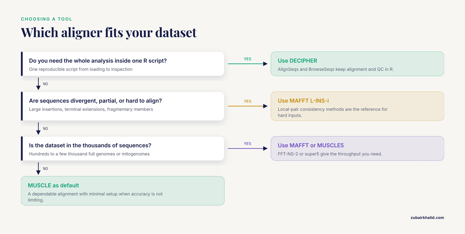
DECIPHER is the only one of the three that runs entirely inside R as a Bioconductor package, MAFFT is the accuracy benchmark for hard nucleotide and protein alignments, and MUSCLE is the fast, low-friction generalist. The practical rule of thumb: use DECIPHER when you want to stay in R end to end and visually inspect every alignment, use MAFFT when alignment quality is the limiting factor or your dataset is large, and use MUSCLE when you want a dependable alignment with minimal setup and you are not chasing the last few percent of accuracy. If you are still deciding between decipher or muscle for a small project, either will do the job, and the difference will usually matter less than your choice of tree model and outgroup.
This article compares the three aligners on their own terms, puts them side by side in a table, walks through real R code for each, and lays out the scenarios where the choice actually changes your result. Everything here assumes a standard R for bioinformatics setup with Bioconductor available, which is covered in any introductory Bioconductor tutorial and summarized briefly below.
Where Alignment Fits in a Phylogenetics Workflow
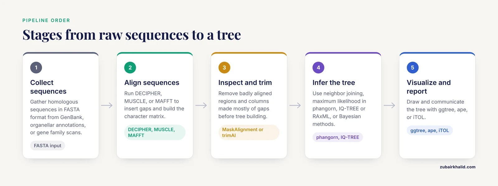
Multiple sequence alignment (MSA) is the step that turns raw homologous sequences into a character matrix. A phylogeny program such as IQ-TREE, RAxML, MrBayes, or phangorn in R can only infer relationships if it assumes that position 100 in sequence A is homologous to position 100 in sequence B. The aligner creates that assumption by inserting gaps. Every downstream step, including the substitution model, bootstrap support, and divergence time estimates, inherits whatever errors the alignment introduced.
Published studies make the stakes concrete. Chloroplast phylogenomics of the rose relative Rosa platyacantha aligned chloroplast genomes spanning 157,133 bp with 132 annotated genes to resolve relationships within Rosa [1]. Mitochondrial phylogenetics of the barn swallow complex aligned 580 complete mitochondrial genomes across subspecies and twelve related Hirundo species to identify five major haplogroups and revise the species' evolutionary history [2]. Comparative work across 1,740 chromosome-level Pseudomonas genomes built phylogenies to trace the distribution of quorum sensing regulators [3]. In each case, the alignment step sat between raw sequences and the final tree, and a poor alignment at that step would have produced confident support values for a wrong tree.
A typical R-based phylogenetics workflow has five stages:
- Collect homologous sequences in FASTA format, from GenBank downloads, organellar genome annotations, or gene family scans.
- Align the sequences with DECIPHER, MUSCLE, or MAFFT.
- Inspect and trim the alignment, removing badly aligned regions and columns made mostly of gaps.
- Infer a tree with distance methods (neighbor joining), maximum likelihood (phangorn, IQ-TREE, RAxML), or Bayesian methods (MrBayes).
- Visualize and communicate the tree with ggtree, ape, or iTOL.
The aligner you pick in stage 2 does not have to be written in R. What matters is that the alignment file you feed into stage 3 is reproducible, of known quality, and appropriate for your data type.
The Three Aligners on Their Own Terms
DECIPHER: Alignment Native to R
DECIPHER is a Bioconductor package written by Erik Wright and colleagues. Its central design decision is that sequences live in an SQLite database on disk and all operations, including alignment, work through that database. This matters most for large datasets, because the database design lets DECIPHER work with thousands of bacterial genomes, plasmids, or long organellar genomes without holding every byte in memory at once.
The core aligner is AlignSeqs(), which handles nucleotide sequences, including long ones such as whole chloroplast and mitochondrial genomes. It uses a profile-based progressive strategy followed by iterative refinement, guided by a position-independent scoring function that rewards consistency with the emerging multiple alignment rather than only pairwise similarity. You control the compute budget with the iterations and refinements arguments. Two related functions cover special cases:
AlignTranslation()aligns protein translations and back-translates to the DNA alignment, which prevents frameshift-inducing gaps in coding sequences.AdjustAlignment()re-optimizes an existing alignment against the scoring function, useful for polishing an alignment imported from another tool.
DECIPHER's killer feature for phylogenetics work is BrowseSeqs(), an HTML viewer that opens in your browser and colors the alignment by base, by translation, or by similarity. Alignment errors that are invisible in a flat FASTA file, such as a single sequence slipped out of frame or a duplicated block of bases, jump out immediately in the viewer. No external aligner offers an inspection tool this tightly coupled to the alignment step.
The costs are speed and breadth. DECIPHER is slower than MAFFT on most inputs, and its strength is nucleotide alignment, particularly long nucleotide sequences, rather than the difficult protein alignments where MAFFT's local-pair methods dominate. DECIPHER also carries its own convention that sequences are stored and aligned in the orientation 5' to 3' of the sense strand, so reverse-complement handling must be considered before aligning mixed-orientation data.
A minimal DECIPHER session looks like this:
library(Biostrings)
library(DECIPHER)

# Load sequences and keep only the accession as the name
seqs <- readDNAStringSet("cp_genomes.fa")
names(seqs) <- sub(" .*$", "", names(seqs))

# Align with iterative refinement
aln <- AlignSeqs(seqs, processors = NULL)

# Refine further if the score had not converged
aln <- AdjustAlignment(aln)

# Inspect in the browser, then export
BrowseSeqs(aln)
writeXStringSet(aln, "decipher_aln.fa")
Two practical notes on the score. AlignSeqs() prints an alignment score as it runs, and the manual advises checking that the score has stopped improving across runs, because a score still climbing means the iterative refinement has not settled. Also, the score is relative to your dataset, so there is no universal "good score" threshold to chase.
MUSCLE: The Fast Generalist
MUSCLE, developed by Robert Edgar, has been a default aligner in countless pipelines for two decades. Version 3.8, still widely installed, runs a progressive alignment followed by iterative refinement of the whole alignment and is famously fast. Version 5, released in 2021, rebuilt the program around a probabilistic consensus model and added the super5 algorithm for datasets in the millions of sequences, where MUSCLE5 trades a small amount of accuracy for very large speed gains.
MUSCLE's virtues are simplicity and predictability. A single command aligns a FASTA file:
muscle -align cp_genomes.fa -output muscle_aln.faVersion 3.8 uses different flags:
muscle -in cp_genomes.fa -out muscle_aln.faFrom R, you can call MUSCLE three ways. The Bioconductor package msa bundles MUSCLE as a compiled backend, so msa(seqs, method = "Muscle") works with no external installation, which makes it the lowest-friction option for a Windows laptop where configuring command-line tools is annoying. The ape package provides muscle(), which shells out to a MUSCLE binary on your PATH. And system2() calls any binary directly.
The honest tradeoff is accuracy on hard inputs. For closely related, clean, full-length sequences, MUSCLE output is usually fine for tree building. For divergent sequences, partial sequences, or alignments dominated by repeats, refinement-based methods such as MAFFT L-INS-i or DECIPHER tend to hold up better. MUSCLE also gives you far less help in evaluating its own output. There is no equivalent of BrowseSeqs(), so quality control moves to separate steps such as trimming or visual inspection in other software.
MAFFT: The Accuracy Benchmark
MAFFT, developed by Kazutaka Katoh and colleagues, is the tool that most benchmark studies and most careful phylogenomic pipelines reach for when alignment quality matters. Its design philosophy is a family of strategies behind one command. -auto inspects your data and picks among them:
- FFT-NS-2 and FFT-NS-i, fast progressive and iterative-refinement methods suited to very large numbers of sequences.
- L-INS-i, which computes pairwise local alignments and uses them to guide the progressive step. This is the strategy of choice for difficult alignments, sequences with large insertions or terminal extensions, and is broadly recommended when you have up to a few hundred sequences.
- G-INS-i, the global-pair analog, for alignments where all sequences are of similar length and globally alignable.
From the command line:
mafft --auto --thread -1 cp_genomes.fa > mafft_aln.faFor maximum accuracy on a small, difficult set:
mafft --localpair --maxiterate 1000 --thread -1 cp_genomes.fa > mafft_linsi.faInside R, the common pattern is system2(), which keeps the whole pipeline in one script:
system2("mafft",
        c("--auto", "--thread", "-1", "cp_genomes.fa"),
        stdout = "mafft_aln.fa")
MAFFT does not come with an R-native viewer, but it is easy to read the output back with Biostrings and pass it to BrowseSeqs() from DECIPHER, which is a hybrid workflow many people use. MAFFT also reports a normalized sum-of-pairs score in its log output, which is useful for verifying that the alignment is internally consistent.
The costs of MAFFT are the external dependency and the decision burden. You need the binary installed and on your PATH, and you need to know which strategy fits your data, though -auto makes a reasonable choice for you and, per the MAFFT documentation, tends to select L-INS-i for smaller inputs on the order of up to a couple hundred sequences.
Side-by-Side Comparison
| Attribute | DECIPHER | MUSCLE | MAFFT |
|---|---|---|---|
| Environment | Native R package, Bioconductor | Standalone binary, callable from R via msa, ape, or system2 | Standalone binary, callable from R via system2 |
| Installation | install.packages via BiocManager, no external binary | Binary install, or zero-install through Bioconductor msa | Binary install required, easy on macOS (Homebrew) and Linux (apt, conda) |
| Best-known strength | Long nucleotide alignment, database-scale workflows, in-browser visual QC | Speed, simplicity, reliable all-purpose alignments | Highest accuracy on difficult alignments, excellent scalability from tens to millions of sequences |
| Algorithm class | Progressive alignment with iterative refinement against a conformational scoring function | Progressive plus iterative refinement (v3.8), probabilistic consensus and super5 (v5) | Progressive variants plus consistency and local-pair refinement (L-INS-i, G-INS-i) |
| Nucleotide vs protein | Strong on nucleotide, supports protein and RNA, AlignTranslation for coding DNA | Both, nucleotide and protein | Both, with local-pair protein methods considered reference-grade |
| Very large datasets | Good, database-backed, but slower per sequence | Excellent with MUSCLE5 super5 | Excellent with FFT-NS-2,, auto scales well |
| Visual quality control | BrowseSeqs in-browser viewer, best in class | None built in | None built in |
| Reproducibility story | R session records version, parameters, and seed-able behavior in one script | Good, single command with fixed version | Good, single command with fixed version and strategy |
| Typical role in a phylogenetics project | End-to-end alignment and QC inside R, coding gene alignment | Quick alignments in pipelines with minimal setup | Reference-quality alignments feeding ML tree inference |
The Criteria That Decide Real Choices
Dataset Size and Sequence Type
Size drives the decision first. For a handful to a few hundred sequences, all three tools finish in seconds to minutes and you should weight accuracy and inspection tools instead. A gene family study, such as the characterization of 97 leucine-rich repeat containing proteins in the Manila clam, which built phylogenies of the RpLRRC members and tested their expression responses to Vibrio alginolyticus challenge, sits squarely in this range [4]. At that scale you can afford L-INS-i, or DECIPHER with generous iterations, and you should visually inspect the result.
For hundreds to a few thousand full genomes or mitogenomes, throughput starts to matter. The barn swallow study's 580 complete mitochondrial genomes [2] and the Pseudomonas study's 1,740 chromosome-level genomes [3] are the kind of input where MAFFT with -auto or FFT-NS-2, or MUSCLE5 with super5, are the natural picks. DECIPHER can operate at this scale because of its database architecture, but expect longer runtimes than the other two.
Sequence type is the second axis. For whole chloroplast or mitochondrial genomes, nucleotide aligners dominate, and DECIPHER was designed with exactly these long nucleotide inputs in mind. A chloroplast genome such as the 157,133 bp R. platyacantha sequence [1] or a mitochondrial genome such as the 658,161 bp two-molecule Rhododendron simsii var. putuoense mitogenome [5] is a realistic DECIPHER target. For protein-coding gene phylogenies, the better question is whether to align the nucleotides or the proteins, which is covered below.
Accuracy Requirements
When the tree is the main result of the paper, alignment quality deserves the most conservative choice. MAFFT L-INS-i is the widely used reference for difficult protein alignments, and MAFFT generally has the strongest reputation in benchmark literature. DECIPHER holds its own on nucleotide data, especially long organellar genomes, and its scoring function plus iterative refinement is specifically built to reduce alignment error on such inputs. MUSCLE is a sound default that occasionally underperforms the other two on divergent or fragmentary sequences.
A defensible practice used by careful groups is to align with two methods and compare. If MAFFT and DECIPHER agree on column boundaries across most of the alignment, confidence goes up. If they disagree substantially, the disagreement regions are exactly where you should look manually before trusting a tree built from them. This cross-check costs little and catches the errors that would otherwise silently propagate into support values.
Staying in R
If the whole project should live in one reproducible R script, DECIPHER has no peer among the three. Everything from loading sequences to inspecting the final alignment happens inside R, with Bioconductor's package versioning recording the tool version implicitly. This matters for teaching, for lab notebooks, and for anyone running the Bioconductor tutorial style of workflow where one script is the entire analysis. A good illustration of R-centric phylogenetic tooling is the phylostratr package used by the MaizeGDB Phylostrata Tool, which the developers updated specifically to keep the R workflow robust against taxonomic database changes, and whose scripts are distributed through GitHub for other researchers [6].
MAFFT and MUSCLE break the single-environment property but remain scriptable. Wrapping them with system2() inside an R Markdown or Quarto document keeps the analysis narrated and rerunnable, and recording the binary version in the script header is enough for most journals. The Bioconductor msa package restores single-environment behavior for MUSCLE specifically, at some cost in flexibility.
Coding Genes and Frameshifts
For protein-coding sequences, aligning nucleotides directly risks introducing gaps of one or two bases, which creates artificial frameshifts and nonsense downstream. Two solutions exist. MAFFT has a back-translation mode for this exact purpose. In R, DECIPHER's AlignTranslation() takes the DNA sequences, translates them, aligns the proteins, and returns a DNA alignment in which all gaps have lengths that are multiples of three. This is the standard fix and it is trivial to apply:
aln <- AlignTranslation(seqs, readingFrame = 1, type = "DNAStringSet")This matters whenever your phylogeny is built from individual genes rather than whole genomes. Many organellar studies concatenate gene alignments, and gene sets there are large. The R. platyacantha chloroplast study annotated 132 genes [1], the R. simsii var. putuoense mitogenome encodes 33 protein-coding genes [5], and the Arabis takesimana mitogenome contains 34 protein-coding genes among 58 annotated genes total [7]. Each of those protein-coding genes, when individually aligned for a concatenated analysis, benefits from translation-aware alignment.
Pre-Alignment Cleanup
None of the three aligners fixes bad input. Sequences with inverted orientation, duplicated regions, or contamination degrade any alignment. Within the DECIPHER ecosystem, CorrectFrameshifts() can detect and repair frameshifts and wrong orientation in nucleotide sets, which is a meaningful advantage when assembling sequences from heterogeneous sources. An Arabis mitogenome study that identified a 5.15 kb mitochondrial plastid DNA insertion carrying intact plastid tRNA genes and part of rrn18 [7] illustrates the kind of transferred sequence that can confound naive alignment and tree inference if not handled deliberately.
End-to-End Worked Workflows
Workflow 1: Chloroplast Genome Phylogeny Entirely in R
This workflow mirrors the design of published chloroplast phylogenomic studies such as the Rosa platyacantha analysis [1].
library(Biostrings)
library(DECIPHER)
library(phangorn)
library(ape)

# 1. Load whole chloroplast genomes
cp <- readDNAStringSet("rosaceae_cp.fa")
names(cp) <- sub(" .*$", "", names(cp))

# 2. Align
cp_aln <- AlignSeqs(cp, processors = NULL)

# 3. Inspect and refine
BrowseSeqs(cp_aln)
cp_aln <- AdjustAlignment(cp_aln)

# 4. Mask poorly aligned columns
cp_aln_masked <- MaskAlignment(cp_aln)

# 5. Build a distance tree, then ML
cp_phyDat <- phyDat(as(cp_aln_masked, "DNAbin"), type = "DNA")
dm <- dist.ml(cp_phyDat)
nj_tree <- NJ(dm)
fit <- pml(nj_tree, cp_phyDat)
fit_gtr <- optim.pml(fit, model = "GTR", rearrangement = "stochastic")

# 6. Bootstrap support
bs <- bootstrap.pml(fit_gtr, bs = 100)
plotBS(fit_gtr$tree, bs, type = "phylogram")
The masking step in stage 4 is where alignment quality and tree quality connect. Highly variable regions with many gaps, such as the intergenic spacers that showed high nucleotide diversity around ycf3-trnS-GCU in the Rosa study [1], contribute phylogenetic signal but also the most alignment uncertainty. Masking lets you test whether the tree topology is stable with and without those regions.
Workflow 2: MAFFT Alignment Feeding an R Tree
This pattern fits a mid-size protein or nucleotide set where accuracy is the priority.
# Alignment stage, outside R's memory
system2("mafft",
        c("--auto", "--thread", "-1", "lrrc_proteins.fa"),
        stdout = "lrrc_linsi.fasta")

# Tree stage, back in R
library(Biostrings)
library(phangorn)
library(ape)

aa <- readAAStringSet("lrrc_linsi.fasta")
names(aa) <- sub(" .*$", "", names(aa))
aa_phy <- phyDat(as(aa, "AAbin"), type = "AA")
dm <- dist.ml(aa_phy)
tree <- NJ(dm)
fit <- pml(tree, aa_phy)
fit_jtt <- optim.pml(fit, model = "JTT", rearrangement = "stochastic")
A gene family set such as the clam RpLRRC proteins [4] is a realistic input here. The same pattern scales upward. For the 580 mitochondrial genomes of the barn swallow study [2], you would replace -auto with an explicit fast strategy and partition per gene, but the R-side code stays identical.
Workflow 3: MUSCLE Through Bioconductor msa
The lowest-friction path, useful on machines where installing external binaries is impractical:
library(Biostrings)
library(msa)

seqs <- readDNAStringSet("barcoding.fa")
msa_result <- msa(seqs, method = "Muscle",
                  order = "input")
aln <- as(msa_result, "DNAStringSet")
writeXStringSet(aln, "muscle_msa_aln.fa")
The order = "input" argument preserves your sequence order in the output, which keeps downstream bookkeeping simple when sequences have metadata keyed by input order.
Worked Scenarios
Scenario A: Ten COI Barcodes for a Species Identification Check
All three tools give the same answer in seconds. Use DECIPHER in R so you can BrowseSeqs() the alignment and spot any sequence in the wrong orientation or with a stop codon from a sequencing error. Frameshift detection in DECIPHER is directly relevant here because a single indel from a sequence read error shows up as a frameshift. The tree itself, a quick neighbor joining with Kimura or TN93 distances, is not sensitive to the aligner at this scale.
Scenario B: Fifty Chloroplast Genomes for a Genus-Level Tree
This is the DECIPHER showcase. Whole chloroplast genomes are long, collinear, and nucleotide-based, which fits AlignSeqs() directly. The workflow is scriptable end to end, BrowseSeqs() catches assembly errors such as an inverted repeat boundary misplaced in one genome, and AlignTranslation() handles the individual genes if you want a concatenated gene-by-gene analysis rather than a whole-genome alignment. Published chloroplast phylogenies, including the Rosa work [1], are built from exactly this kind of input.
Scenario C: Two Thousand Mitochondrial Genomes for a Population-Level Phylogeny
Throughput now dominates. MAFFT with -auto on the whole genome or per-gene partitions, or MUSCLE5 with super5, are the pragmatic choices. The barn swallow study is the scale reference, with 580 complete mitogenomes resolved into five major haplogroups and a revised southern African origin for the species [2]. At this scale, per-gene alignment followed by concatenation is usually preferable to whole-genome alignment, because gene boundaries give natural partitions for substitution models.
Scenario D: A Protein Family with Divergent Members and Partial Sequences
MAFFT L-INS-i first, DECIPHER as a cross-check, MUSCLE as a quick sanity check. Divergent and partial sequences are where naive progressive alignment produces spurious column matches, and consistency-based local-pair methods in MAFFT are designed for this case. A quorum sensing regulator phylogeny across the genus Pseudomonas, where complete LuxI/R systems show patchy lineage-dependent distribution and LuxR solo regulators are pervasive and expanded, represents the kind of analysis where regulator families include many divergent parologs and alignment choice visibly affects the gene tree [3].
Common Mistakes and Limitations
Aligning nucleotides when proteins are the safer target. For divergent protein-coding genes, direct nucleotide alignment inflates gap counts and produces frameshifts. Align the translation and back-translate, with AlignTranslation() in DECIPHER or MAFFT's back-translation mode. This is the single most common fixable error in gene-based phylogenetics.
Trusting an alignment you never looked at. Every aligner makes errors, and errors concentrate in repetitive regions, near terminal ends, and around long insertions. Open the alignment in a viewer before tree building. DECIPHER's BrowseSeqs() makes this a thirty-second habit. Skipping inspection is how a single misassembled genome silently shifts an entire clade.
Ignoring biological processes that alter the sequence. RNA editing changes mitochondrial transcript sequences relative to the gene model, and plant mitogenomes carry substantial editing loads. The Rhodobryum laxelimbatum study documented 189 RNA editing sites in the mitogenome and 608 in the chloroplast [8], and the R. simsii var. putuoense analysis predicted 463 editing sites in the mtDNA [5]. If you align genomic sequences while your annotations assume edited transcripts, mismatches at editing sites can be misread as substitutions. Decide deliberately whether your gene sequences are genomic or cDNA-derived and be consistent across taxa.
Confusing alignment speed with pipeline speed. The aligner is usually not the bottleneck in a phylogenetic analysis. Model selection, bootstrapping, and divergence time estimation take far longer. Choosing a faster aligner to save minutes while spending days on tree inference is a misallocation.
Forgetting that alignment is a hypothesis of homology. An alignment is not truth, it is a model. Sensitivity analyses, rebuilding the tree after masking uncertain columns, excluding fast-evolving sites, or switching aligners, tell you whether your conclusions survive reasonable alternative alignments. Studies that report only one alignment and one topology overstate their certainty.
Mixing aligner versions across a project. MUSCLE 3.8 and MUSCLE 5 produce different alignments, and MAFFT's behavior depends on the selected strategy. Record the exact version and strategy in your script. A paper's methods section that says "aligned with MUSCLE" without a version is not reproducible.
One general limitation deserves a plain statement. Alignment and tree building are computational judgments that do not replace biological judgment, and any conclusion about a specific organism or clinical or husbandry question needs domain expertise on top of the phylogeny.
Frequently Asked Questions
Which tool should a beginner start with?
Start with DECIPHER if you already work in R, because installation is one BiocManager call and the visual QC tool teaches you what alignments look like. Add MAFFT once your datasets grow or your sequences become divergent.
Is DECIPHER as accurate as MAFFT?
There is no universal answer, and honest practice is to test both on your data. DECIPHER's design targets long nucleotide sequences, where it is competitive, while MAFFT's local-pair strategies are the usual reference for difficult protein alignments. Comparing the two alignments on your own dataset is cheap and settles the question for your specific input.
Can I run MAFFT or MUSCLE from inside R on Windows?
Yes. Install the binary and add its directory to your system PATH, then call it with system2(). Alternatively, use the Bioconductor msa package, which bundles MUSCLE so no external installation is needed.
Should I align nucleotides or translated proteins for a coding gene?
Align the proteins and back-translate to DNA for anything beyond closely similar sequences. This guarantees gaps in multiples of three, preserves the reading frame, and generally produces a more accurate alignment because amino acid substitution matrices carry more information than nucleotide models over long divergence times.
What does the DECIPHER alignment score mean?
The score is a relative measure of how well the current alignment fits DECIPHER's scoring function, not an absolute quality grade. The number to watch is convergence. If the score still rises when you rerun alignment with more iterations, the refinement has not settled and you should continue.
How do I trim an alignment before building a tree?
In R, MaskAlignment() from DECipher masks columns dominated by gaps or by rare signal. Standalone tools such as trimAl and BMGE are common alternatives, and any trimming step should be reported in your methods with the exact parameters, because aggressive trimming can remove real phylogenetic signal along with noise.
Sources
- Characteristics, comparative genomics, and phylogenetic analysis of the chloroplast genome of Rosaplatyacantha.
- Mitogenomes Reveal Novel Phylogeographic Patterns and Temporal Evolutionary History of Barn Swallows and Close Relatives.
- Ecological and evolutionary diversification of LuxI/R quorum sensing and LuxR solo regulators in Pseudomonas.
- Genome-wide identification and comparative analysis of Leucine-Rich Repeat Containing (LRRC) gene and their expression responses to Vibrio alginolyticus infection in the Manila clam (Ruditapes philippinarum).
- Characterization of the complete mitochondrial genome of Rhododendron simsii var. putuoense and its comparative evolutionary analysis.
- MaizeGDB Phylostrata Tool: exploring evolutionary origins of maize proteins.
- Mitochondrial Genome of the Korean Endemic Arabis takesimana (Brassicaceae): Addition to the Genomic Resources and Evolutionary Insights.
- Mitochondrial Genome Characteristics of Rhodobryum laxelimbatum and Comparative Analysis of RNA Editing and Codon Usage Bias With the Chloroplast Genome.