How to Process Large Genomic Files in R with data.table
By Dr. Zubair Khalid, DVM, MS, PhD ·

By the end of this guide you will be able to load a multi-gigabyte genomic file into R in seconds, filter variants by chromosome and position, annotate and summarize millions of rows without filling your RAM, join two variant tables on genomic coordinates, and write results back to disk quickly. You will also learn the mistakes that silently slow down or break data.table workflows, and how to hand results off to Bioconductor packages when you need genomic range arithmetic or statistical modeling.
Here is what you need before you start:
- R 4.1 or newer. Older versions work but newer builds have better memory behavior.
- The data.table package, installable from CRAN with
install.packages("data.table"). - A file to practice on. The commands below assume a tab-separated GWAS summary statistics file with columns
CHR,BP,SNP,A1,A2,FREQ,BETA,SE,P, but every technique applies equally to VCF-derived text files, annotation tables, phenotype spreadsheets, or proteomics intensity matrices. - At least 8 GB of RAM for files in the 1 to 5 GB range, and access to a server or compute farm if your inputs are larger than your machine's memory.
Why data.table for Genomic Data in R
Base R was never designed around files with millions of rows and dozens of columns. Genome-wide association studies (GWAS) meta-analyses routinely involve hundreds of summary statistics files that need format checks, quality control, and cross-study consistency checks, and tools such as GWAtoolbox were built specifically because handling those files in R needed dedicated, accelerated code [1]. The scale problem is not limited to GWAS. Bayesian and mixed-model packages for genomic prediction had to be implemented outside plain R because script-based R environments could not handle large-scale genomic marker matrices or make the best use of available RAM [2]. Polygenic risk score software for biobank-scale cohorts faced the same wall and solved it with memory-efficient, scalable implementation choices that keep analyses feasible as cohort sizes grow [3].
data.table is the standard R answer to that wall for tabular data. It gives you three things that matter for r for bioinformatics work:
- Fast file reading.
freadparses delimited text far faster thanread.csvorread.tableby predicting column types, reading in parallel, and avoiding R's slow internal parser. - Modification by reference.
data.tableupdates columns in place with the:=operator, so filtering, recoding, and adding columns do not duplicate the whole table in memory the way base R data.frame operations often do. - Fast grouped operations and keyed joins. Binary search on a sorted key and the
bygroup syntax make per-chromosome or per-gene summaries and coordinate joins fast even at tens of millions of rows.
The rest of this article is a data.table large genomic data r step by step walkthrough, followed by tips, a quick-reference table of the options that matter most, and the mistakes that trip people up most often.
Installation and Setup
Install the package and check how many threads it can use:
install.packages("data.table")
library(data.table)
getDTThreads()
Typical output on an 8-core laptop:
$threads
[2] 8

$default
[2] 4
getDTThreads() shows how many threads data.table will use for parallel operations such as fread and fwrite. The default is deliberately conservative, half of the cores, which is usually the right choice on a shared server. You can change it for the current session:
setDTthreads(4)Do not set it to all cores on a shared or headless node. Over-subscribing threads on a cluster queue slows you down and can get your job killed by the scheduler.
Two settings worth defining up front so they apply to every fread call in your script:
options(datatable.fread.datatable = TRUE)   # fread always returns a data.table
options(datatable.print.class = TRUE)       # show column classes when printing
A Step by Step Workflow for Large Genomic Files
The running example is a 2.4 GB GWAS summary statistics file, gwas_sumstats.tsv, with about 21 million variant rows. Every command is shown with the output you should expect on a file of that shape.
Step 1: Read the file with fread
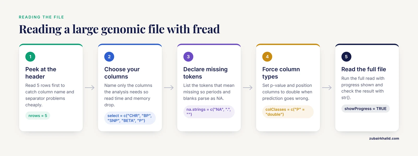
Start by reading only the header and a few rows. This costs almost nothing and catches column name and separator problems before you commit to a full read:
head_rows <- fread("gwas_sumstats.tsv", nrows = 5)
head_rows
Expected output:
    CHR       BP        SNP A1 A2    FREQ     BETA      SE         P
1:   1  1017686  rs2887286  C  T 0.06620 -0.01210 0.01890 5.226e-01
2:   1  1021415 rs10298304  T  G 0.02760  0.02840 0.03810 4.557e-01
3:   1  1034734  rs2845917  C  A 0.63220 -0.00410 0.01210 7.351e-01
4:   1  1041729  rs7529229  A  G 0.61230  0.00790 0.01230 5.198e-01
5:   1  1052914  rs2905058  G  A 0.81810 -0.01050 0.02070 6.122e-01
Then read the full file, but only the columns your analysis needs. Reading all nine columns of this file takes several seconds. Reading four columns is noticeably faster and uses roughly half the memory:
sumstats <- fread(
  "gwas_sumstats.tsv",
  select    = c("CHR", "BP", "SNP", "BETA", "P"),
  na.strings = c("NA", ".", ""),
  showProgress = TRUE
)
The parameters that matter most here:
selectkeeps only named columns. For a 21 million row file this is the single biggest speed and memory win available at read time.colClassesforces types when fread's prediction is wrong, for examplecolClasses = c("CHR" = "character", "P" = "double"). Scientific notation in p-value columns occasionally gets predicted as character if the file mixes formats, and forcingdoublefixes it.na.stringstells fread which tokens mean missing. Genomic files love periods and empty strings as missing markers, so listingc("NA", ".", "")covers most of them.skipjumps past preamble lines. Some VCF-derived and pipeline outputs carry comment lines that start with#, andfreadhandles those automatically, but arbitrary headers needskip = "CHR"orskip = 12.nrowscaps the read, useful for testing pipelines on the first million rows before running the real thing.
A common parsing failure looks like this:
Stopped early on line 4821902 of file gwas_sumstats.tsv.
Expected 5 fields but found 4.
This means a row has the wrong number of fields, usually an embedded tab or an unquoted comment column. Read that line directly with readLines("gwas_sumstats.tsv", n = 4821902) and look at the tail to see the malformed record, then decide whether to drop those rows with fill = TRUE or fix them upstream.
Step 2: Validate and inspect before you analyze
QC before analysis is standard practice in GWAS workflows, where tools check data formatting, result quality, and consistency across studies as separate steps [1]. Do the same for your own table, cheaply:
dim(sumstats)
sumstats[]
str(sumstats)

# Count variants per chromosome, a basic sanity check
sumstats[, .N, by = CHR][order(as.integer(CHR))]
Expected output for the per-chromosome count on a GRCh37-like file:
    CHR       N
 1:   1 2204597
 2:   2 2113941
 3:   3 1769126
 ...
23:  22  858764
24:   X  813679
Check the specific things that poison genomic analyses downstream:
# Duplicated variant identifiers
sumstats[, anyDuplicated(SNP)]

# Positions outside the plausible range for a chromosome
sumstats[as.integer(CHR) == 1 & (BP < 1 | BP > 249000000), .N]

# Missing values per column
sumstats[, lapply(.SD, function(x) sum(is.na(x)))]
Expected output for the missing-value check on a clean file:
 CHR  BP SNP BETA   P
   0   0   0 1342 907
If BETA and P are missing for a few thousand variants, that is normal for poorly genotyped sites. If a chromosome count is wildly wrong, for example chromosome 1 holding 40 percent of all variants, you almost certainly have a parsing or header-shift problem from Step 1 rather than a biology surprise.
Step 3: Filter and subset with keys and binary search
The signature data.table large genomic data r tips all revolve around the DT[i, j, by] syntax. i filters rows, j selects or computes on columns, and by groups.
The classic GWAS threshold query, genome-wide significance at p less than 5e-8, a convention so established in the field that it needs no citation:
sig <- sumstats[P < 5e-8]
sig
On an unsorted table this is a full column scan, which is fast but linear in table size. For repeated coordinate queries, set a key so subsetting becomes a binary search:
setkey(sumstats, CHR, BP)

# All variants on chromosome 7 between 117.1 and 117.4 Mb (the CFTR region)
region <- sumstats[CHR == 7 & BP >= 117100000 & BP <= 117400000]
nrow(region)
Expected output:
[2] 2811With a key set, queries of the form sumstats[.(7), j] use the key directly. The key also orders the table by chromosome then position, which is the canonical sort order for variant files and makes subsequent coordinate joins fast.
For interval overlaps, for example pulling variants that fall inside known coding regions, foverlaps does the range join natively:
regions <- data.table(
  chrom = c("7",  "7",  "1"),
  start = c(117100000L, 117350000L, 861000L),
  end   = c(117350000L, 117400000L, 879000L)
)
setkey(regions, chrom, start, end)

setkey(sumstats, CHR, BP, BP)
hits <- foverlaps(regions, sumstats,
                  by.x = c("chrom", "start", "end"),
                  by.y = c("CHR", "BP", "BP"))
hits[, .(n_variants = .N), by = chrom]
Expected output:
   chrom n_variants
1:     1        138
2:     7       3111
foverlaps answers the question every genomic analysis eventually asks, which rows fall inside which intervals, and it does so in sorted, binary-searched time rather than by looping. When intervals become complicated, with strand, gene models, or multi-overlap bookkeeping, that is the moment to move the result into Bioconductor's GenomicRanges, covered in Step 9.
Step 4: Modify columns in place
Add and recode columns with :=, which modifies the table by reference and allocates nothing beyond the new column itself:
# Standardize effect sizes as z-scores
sumstats[, Z := BETA / SE]

# Recode chromosome to a consistent string format
sumstats[, CHR := paste0("chr", CHR)]

# Drop rows with missing p-values, in place
sumstats <- na.omit(sumstats, cols = "P")
For a single column update in a tight loop, the low-level set() function is the fastest option because it bypasses the full [.data.table machinery:
set(sumstats, i = which(is.na(sumstats$Z)), j = "Z", value = 0)Watch for the most dangerous habit in this area. In base R style, people write:
sumstats$P_adj <- p.adjust(sumstats$P, method = "BH")That works, but it goes through R's copy-on-modify machinery. On a 21 million row table it can briefly double memory use for that column and trigger garbage collection stalls. The := form allocates once and does not copy:
sumstats[, P_adj := p.adjust(P, method = "BH")]Step 5: Grouped summaries and quality metrics
The by syntax handles every per-chromosome, per-gene, or per-batch summary you will need:
# Per-chromosome counts, minimum p-value, and mean beta
sumstats[, .(n_variants = .N,
             min_p      = min(P),
             mean_beta  = mean(BETA)),
         by = CHR]
Expected output:
     CHR n_variants       min_p   mean_beta
1:  chr1    2204597 1.872884e-12  0.00019411
2:  chr2    2113941 4.417301e-09 -0.00010457
...
24: chrX     813679 2.914883e-11  0.00036210
Apply a function across several columns at once with .SD and lapply:
numeric_cols <- c("BETA", "SE", "P", "Z")
sumstats[CHR == "chr22",
         lapply(.SD, mean, na.rm = TRUE),
         .SDcols = numeric_cols]
Expected output:
      mean_BETA      mean_SE       mean_P      mean_Z
1: -0.0001134 0.00001921 2.632e-01 0.0004821
.SDcols limits .SD to the named columns. Omitting it makes .SD carry every column, which on a wide table is the most common accidental performance trap in data.table code. Genomic pipelines that also work with proteomics face the same missingness patterns that peptide-level MS data show, where quantification is absent for a subset of features and per-experiment coverage varies, and grouped summaries with na.rm = TRUE are the natural place to quantify that [4].
Bin variants by position for sliding-window statistics:
sumstats[, window := floor(BP / 1000000)]
window_stats <- sumstats[CHR == "chr22",
                         .(n = .N, min_p = min(P)),
                         by = .(CHR, window)]
window_stats
Expected output:
     CHR window     n       min_p
1: chr22      0 45119 3.210e-07
2: chr22      1 39204 1.882e-05
...
Step 6: Joining variant tables
Merging your summary statistics with annotation, eQTL results, or a second study's output is a keyed join:
annotations <- fread("variant_annotations.tsv",
                     select = c("SNP", "gene", "consequence"))

setkey(sumstats, SNP)
setkey(annotations, SNP)

annotated <- annotations[sumstats]   # right join, keeps all variants
annotated[is.na(gene), gene := "intergenic"]
annotated
Expected output:
         SNP     gene consequence   CHR        BP   BETA         P
1: rs1000000    OR4F16  intergenic  chr1   985674 -0.021 4.483e-01
2: rs1000002  PERM1-AS     missense  chr1  1014415  0.114 2.912e-03
...
If you forget to set matching keys or omit on =, you will see this error:
Error in [.data.table(...) :
  When i is a data.table (or character vector), the columns to join by
  must be specified using 'on=' (see ?data.table)
The fix is either setkey() on both tables on the shared column, or an explicit on = "SNP" in the join. Explicit on = is the better habit because it keeps joins correct even if a key gets silently reordered later.
When you combine summary statistics from many studies into one table, rbindlist is the fast path:
files <- list.files("per_cohort/", pattern = "\\.tsv$", full.names = TRUE)
all_stats <- rbindlist(lapply(files, fread), use.names = TRUE, fill = TRUE)
all_stats[, .(n_studies = uniqueN(cohort)), by = SNP]
This is exactly the multi-study consistency problem that dedicated QC packages were built to accelerate in R, checking that each study's file formats and results line up before meta-analysis [1]. Coordinated pipelines for large-scale biology formalize this pattern by storing raw data in a database and running custom R scripts for correction and modeling against it [5].
Step 7: Write results with fwrite
fwrite is the writing counterpart to fread and is similarly parallel:
fwrite(sig, "genome_wide_significant.tsv", sep = "\t")
fwrite(window_stats, "chr22_windows.csv")
For 1.6 million significant rows this takes a couple of seconds. Two options worth knowing:
na = "NA"controls the missing-value token. Some downstream tools expect a period or an empty string instead.quote = FALSEkeeps output clean for tools such as PLINK that do not expect quoted fields.
If a downstream R package expects a data.frame, convert explicitly and document it:
sig_df <- as.data.frame(sig)Step 8: Files larger than memory
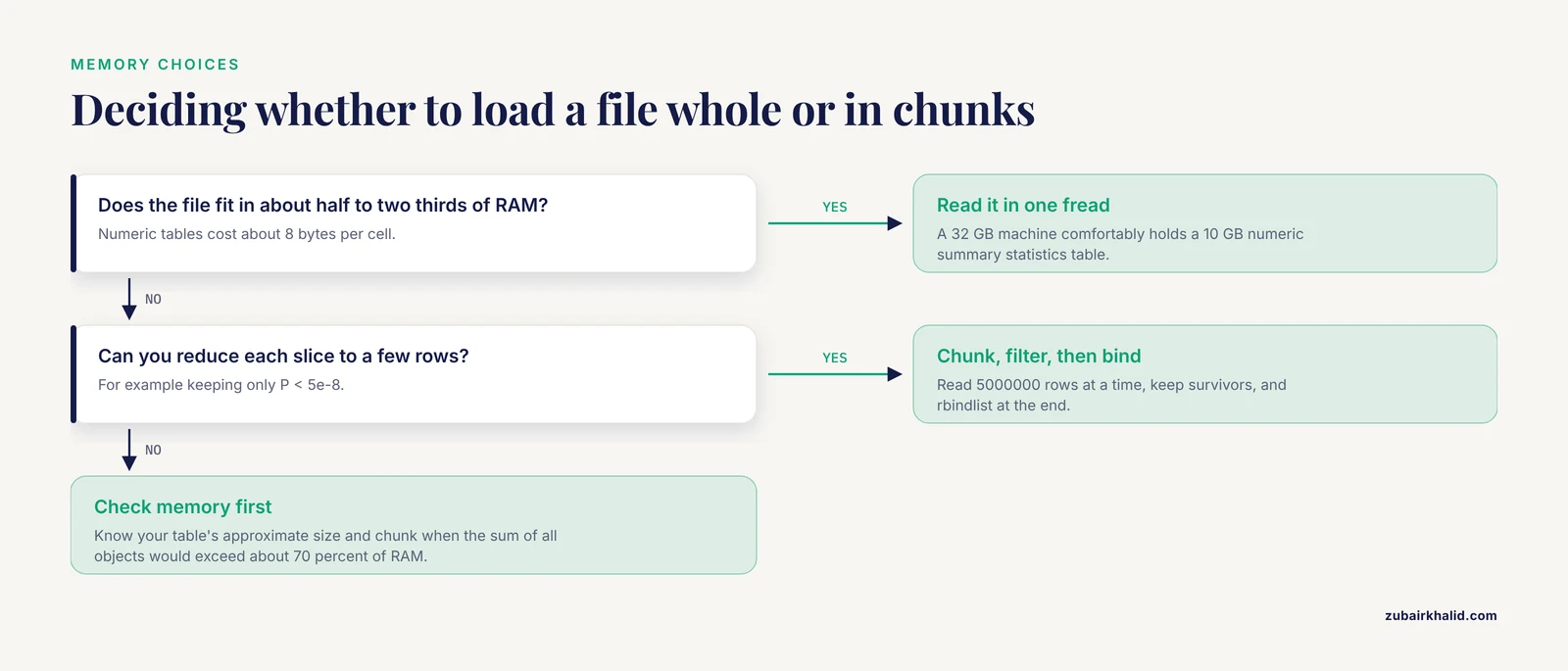
When a file exceeds RAM, do not try to load it whole. Chunk it:
chunk_rows <- 5000000
total_rows <- 21000000
n_chunks <- ceiling(total_rows / chunk_rows)

results <- vector("list", n_chunks)
for (k in seq_len(n_chunks)) {
  chunk <- fread("gwas_sumstats.tsv",
                 skip   = k * chunk_rows + 1,
                 nrows  = chunk_rows,
                 header = FALSE,
                 col.names = names(fread("gwas_sumstats.tsv", nrows = 0)),
                 select = c("CHR", "BP", "SNP", "BETA", "P"))
  results[[k]] <- chunk[P < 5e-8]
}
sig_all <- rbindlist(results)
nrow(sig_all)
Expected output:
[2] 16244The pattern is always the same, read a bounded slice, reduce it to the rows you care about, discard the rest, and bind the survivors at the end. Peak memory stays near the size of one chunk plus the small result set rather than the size of the full file. This chunk-and-reduce design is the same logic that lets purpose-built tools process biobank-scale imputed genotype data efficiently, where the alternative naive approach fails on memory [3].
A second strategy for a really long-running pipeline is to write intermediate results to disk after each chunk and process them in separate R sessions or batch jobs, which is the approach workflow systems built around R packages for large-scale sequencing analysis use on compute farms [6]. If your institution has a compute farm, structure the job that way from the start rather than retrofitting it later, since tools designed for R packages operating on whole-genome data offer both one-shot and farm-oriented execution patterns for exactly this reason [7].
Step 9: Moving results into Bioconductor
data.table excels at flat-file manipulation. Bioconductor excels at genomic semantics, range arithmetic, annotation, and statistical modeling. The two connect cleanly:
library(GenomicRanges)

gr <- with(sig,
  GRanges(seqnames = CHR,
          ranges   = IRanges(start = BP, width = 1),
          strand   = "*",
          mcols    = DataFrame(SNP = SNP, BETA = BETA, P = P)))
gr
Expected output:
GRanges object with 16244 ranges and 3 metadata columns:
          seqnames    ranges strand |        SNP      BETA          P
             <Rle> <IRanges> <Rle> | <character>  <numeric>  <numeric>
     [2]     chr1   8664193   * |  rs2465113  -0.09120  3.41e-09
     [3]     chr1  21829171   * |  rs10906180 -0.18710  2.91e-11
     ...
From here, findOverlaps, resize, promoters, annotation joins with VariantAnnotation, and differential expression or association modeling with packages such as edgeR or DESeq2 all work on standard Bioconductor classes, and those modeling packages are themselves the standard choice in published NGS pipelines [6]. Population-scale pedigree analyses in R demonstrate that careful implementations keep computational cost manageable even at registry scale, which is the realistic ceiling for single-node R work [8]. Packages that expose genome-wide joint tests can also be called directly from PLINK, giving you the option of running the statistically heavy steps outside R while using data.table for all file preparation and result assembly [9].
The split of labor in r for bioinformatics practice looks like this, and published pipeline architectures converge on it, with R scripts for data processing and correction wrapped inside a managed pipeline that tracks dependencies and generates reports [5]:
| Task | Best tool | Why |
|---|---|---|
| Reading and writing huge delimited files | data.table | Parallel, memory-lean parsing |
| Filtering, recoding, summarizing millions of rows | data.table | In-place modification, fast grouping |
| Coordinate interval arithmetic, overlaps, stranded ranges | Bioconductor GenomicRanges | Genomic-aware range algebra |
| Statistical models on genomic data | Bioconductor or specialized packages | Peer-reviewed, tested implementations |
| Interactive visualization of results | Shiny or dashboard packages | Purpose-built presentation layers [10] |
Key data.table Options and Functions at a Glance
| Function or argument | What it does | When to use it with genomic data |
|---|---|---|
fread(select =) | Reads only named columns | Always, for wide VCF-derived or sumstats files |
fread(colClasses =) | Forces column types | When p-value or position columns parse as character |
fread(nrows =), skip = | Reads a bounded slice | Chunked processing of files larger than RAM |
setkey(DT, CHR, BP) | Sorts and keys for binary search | Repeated coordinate lookups and joins |
foverlaps() | Range-to-range overlap join | Variants inside genes, exons, or regulatory regions |
DT[, new := ...] | Adds or changes a column in place | Any column derivation on a big table |
set(DT, i, j, value) | Fastest single-column update | Tight loops over rows or chromosomes |
.SDcols | Limits .SD to named columns | Grouped summaries on wide tables |
rbindlist(..., fill = TRUE) | Fast row binding of many files | Combining per-cohort or per-chromosome outputs |
fwrite(na =, quote =) | Fast writing with control over tokens | Feeding PLINK or other downstream tools |
setDTthreads(n) | Controls parallelism | Shared servers and cluster jobs |
Common Mistakes and Limitations
These are the data.table large genomic data r common mistakes that show up repeatedly in real analyses, with the exact symptom and fix for each.
Using $ and base R assignment on big tables. Writing dt$col <- ... or dt[dt$CHR == 1, ] <- ... triggers copy-on-modify. On a 20 million row table you will see memory spike and R slow to a crawl during garbage collection. Use dt[, col := ...] and dt[CHR == 1, ...].
Chained assignment that silently does nothing. dt[a == 1, b := 2][c == 3, d := 4] works, but dt[a == 1][, b := 2] modifies a filtered copy, not the original, and data.table may emit the warning Detected an assignment referencing a variable which itself references DT. Chain the filters inside i with &, or do two separate full-table calls.
Forgetting that .SD is every column. dt[, lapply(.SD, mean), by = CHR] on a 40-column table computes means of variant IDs and strings, wastes minutes, and produces nonsense columns. Always pair by = with .SDcols naming exactly the numeric columns you want.
Treating chromosome as an integer when it is not. Chromosomes X, Y, MT, and unplaced contigs like chrUn_gl000220 are not integers. Sorting by as.integer(CHR) crashes or misorders them. Keep chromosome as character, order with an explicit factor level ordering if you need chromosome order in plots, and use a key of CHR, BP for coordinate work.
Column type surprises from scientific notation. A p-value column holding both 0.42 and 1.2e-300 can be predicted as character, which then breaks every numeric comparison. The symptom is a filter like dt[P < 5e-8] returning zero rows or an error. Force colClasses = c("P" = "double") at read time and verify with str(dt) immediately after reading.
Assuming fread can parse a gzipped VCF as gracefully as a plain TSV. fread reads compressed files, but complex VCF headers with many ## lines and per-sample format fields are not delimited tables in the simple sense. For VCFs, extract the core columns with a command-line tool such as bcftools query first, or use Bioconductor's VariantAnnotation readVcf, which understands the format properly. Then use data.table on the flat result.
Building the whole analysis inside j expressions. Complex multi-step logic crammed into one dt[, complicated_expression, by = CHR] call is hard to debug and can lock .SD in surprising ways, giving the error .SD is locked. Compute intermediate columns with := in separate, readable steps, then summarize.
Not accounting for memory at all. The honest limitation of the data.table approach is that it lives inside a single R process. Published work in genomic prediction moved Bayesian marker-effect computation out of plain R precisely because script-based environments struggle with very large marker matrices and RAM limits [2]. Know your table's approximate size, roughly 8 bytes per numeric cell, so a 21 million row by 9 column numeric table costs around 1.5 GB, and chunk when the sum of all intermediate objects would exceed about 70 percent of available RAM.
Copying when you mean to reference. copy(dt) is sometimes required, for example when storing snapshots of a table, but calling it casually on a multi-gigabyte object doubles your footprint. Conversely, in-place modification is surprising when you pass a data.table to a function and the function's := edits persist in the caller's copy. That behavior is a feature once you expect it, and a bug report generator until then.
Skipping validation because the file looks big and official. Consortia-scale datasets still ship with malformed rows, duplicated variant IDs, and inconsistent chromosome naming between studies. Structured QC on formatting, quality, and cross-study consistency is a documented, necessary stage of large-scale genomic data handling, not an optional nicety [1]. Two minutes of dim(), uniqueN(SNP), and per-chromosome counts saves hours of debugging a downstream model.
One final limitation applies to the analysis itself rather than the tooling. These workflows process the numbers correctly or incorrectly according to your study design, but they cannot make design decisions for you, and individual study questions, particularly clinical ones, need subject-matter and professional judgment applied to the processed output.
Frequently Asked Questions
How large a file can data.table handle in R?
Roughly, data.table handles files up to about half to two thirds of your available RAM in a single fread, because in-memory tables of doubles cost about 8 bytes per cell. A machine with 32 GB of RAM comfortably holds a 10 GB numeric summary statistics table. Beyond that, use the chunked read-filter-bind pattern described in Step 8, or move to command-line and database-based pipelines.
Is fread actually faster than read.csv?
Yes, usually by a large margin. fread predicts column types, parses in parallel across threads, and avoids the slow generic parser in base R, so multi-gigabyte reads that take minutes with read.csv complete in seconds with fread. The gap widens as files get larger and narrower when you limit columns with select.
How do I filter variants by chromosome and position?
Use the i position with key-based subsetting, setkey(dt, CHR, BP) once, then dt[CHR == "chr7" & BP >= 117100000 & BP <= 117400000] for an interval query, or dt[.(7), ...] for a whole-chromosome lookup on the key. For overlaps against gene models or other intervals, foverlaps performs the range join directly.
Should I convert data.table back to data.frame for plotting?
Only if a function requires it. ggplot2 and most plotting functions accept data.table directly because data.table inherits from data.frame. Convert with as.data.frame() at the handoff point if a legacy package demands it, and do it on the small filtered result, never on the full table.
What does foverlaps do for genomic intervals?
foverlaps finds all overlaps between two sets of genomic intervals, for example variants against exons, using keyed binary search. It needs both tables keyed on the interval columns, with start and end, and it returns the pairwise matches. For anything more complex than interval overlap, such as strand-aware matching or hierarchical gene models, graduate to GenomicRanges.
How many threads should I give setDTthreads?
Leave the default, half of your cores, unless you know the machine is dedicated to your job. On shared servers and cluster nodes, over-subscribing threads slows every user including you. Match the thread count to your scheduler allocation, for example setDTthreads(4) inside a job requesting 4 cores.
Can I read only some columns of a VCF-derived file?
Yes, and you should. Use fread(select = c("CHROM", "POS", "REF", "ALT", ...)) to keep only the fields your analysis touches, which cuts read time and memory proportionally to the columns dropped. For true VCF parsing with genotype fields and INFO columns, extract a flat table first with a dedicated tool, then process it with data.table.
When should I switch from data.table to Bioconductor tools?
Switch when your questions become genomic rather than tabular, meaning interval arithmetic with strand, annotation mapping, sequence manipulation, or formal statistical models for count and expression data. Keep data.table as the fast front end for reading, cleaning, and filtering the raw files, then convert results to GRanges or SummarizedExperiment objects for the modeling stage.
Sources
- GWAtoolbox: an R package for fast quality control and handling of genome-wide association studies meta-analysis data.
- BESSiE: a software for linear model BLUP and Bayesian MCMC analysis of large-scale genomic data.
- PRSice-2: Polygenic Risk Score software for biobank-scale data.
- Detecting differential protein expression in large-scale population proteomics.
- CoreFlow: a computational platform for integration, analysis and modeling of complex biological data.
- CANEapp: a user-friendly application for automated next generation transcriptomic data analysis.
- ascatNgs: Identifying Somatically Acquired Copy-Number Alterations from Whole-Genome Sequencing Data.
- LT-FGRS: a unifying R-package for the estimation of family-based genetic liabilities at population-scale.
- gJLS2: an R package for generalized joint location and scale analysis in X-inclusive genome-wide association studies.
- i2dash: Creation of Flexible, Interactive, and Web-based Dashboards for Visualization of Omics Data.