Data Organization in Bioinformatics Platforms
By Dr. Zubair Khalid, DVM, MS, PhD ·

By the end of this article you will be able to design a bioinformatics project directory that survives reviewer scrutiny, build a machine-readable sample sheet, pin your software environment, run a versioned workflow from raw sequencing reads to a quality-controlled report, verify that outputs are correct, and compare platform options with a clear framework. You will also learn the failure modes that break real projects, with fixes drawn from current literature.
To follow the walkthrough you need a Linux or macOS shell, Miniconda or another Conda distribution, a workflow engine (the walkthrough uses Snakemake and Nextflow), Docker installed and running, Git, and about 20 GB of free disk space for the example. Every command shown runs as written on a standard Unix shell.
What Data Organization in Bioinformatics Platforms Actually Means
A bioinformatics platform is the combination of storage, file formats, metadata, software tools, and workflow machinery that moves data from an instrument to a defensible result. Data organization is the discipline of arranging those pieces so that any analysis can be rerun months later, by you or by a stranger, and produce the same numbers.
The problem has grown with the instruments. High-throughput devices now generate enormous volumes of genetic data at low cost, and that volume of big data makes even basic operations such as choosing informative features in large medical databases a serious organizational challenge [1]. The response from the field has been to build platforms, and a recent review of cancer-focused resources distinguishes four organizing categories, databases, analytical web servers, prediction tools, and integrated analysis platforms, each with different data coverage, analytical capabilities, and limitations [2]. Knowing which category a resource belongs to is itself a data-organization skill, because it tells you what the resource can hold, what it can compute, and what you must bring yourself.
At the concrete end of the spectrum, BILBO (Bioinformatics Integration for Large-scale Biological Operations) is a self-hosted, fully containerized platform that consolidates data acquisition, quality control, alignment, quantification, normalization, differential expression analysis, and publication-ready outputs into standardized workflows within one environment [3]. That single sentence describes the target state of this article, one coherent, reproducible pipeline instead of a folder of loose scripts.
The Four Layers of an Organized Project
Every well-run bioinformatics platform separates data into four layers. Mixing them is the root cause of most reproducibility failures.
- Raw data. Instrument output, immutable, never edited, protected by checksums. Examples are FASTQ files from a sequencer, vendor mass spectrometry files, and microscope image stacks.
- Metadata. The description of every sample, including identifiers, conditions, batch, and file locations, kept in structured tables.
- Processed data. Alignment files, count matrices, quantification tables, and results, all regenerable from raw data plus code.
- Code and environment. Workflows, configuration files, container images, and version records that transform layer 1 into layer 3.
The formats you choose determine how well each layer organizes and scales.
| Data type | Common format | Key organizing property |
|---|---|---|
| Raw sequencing reads | FASTQ (often gzipped) | Four-line records, human inspectable, compresses well |
| Aligned reads | BAM or CRAM | CRAM stores the same information as BAM in less space by referencing a genome |
| Variant calls | VCF or BCF | Tab-delimited, indexable, supports large cohorts |
| Count matrices | TSV, HDF5, Zarr | Binary backends allow chunked access to matrices too large for memory |
| Single-cell and spatial objects | AnnData (H5AD), Zarr stores | Bundles expression, cell metadata, and embeddings in one file |
| Workflows and configs | YAML, CSV, Nextflow or Snakemake files | Plain text, versionable with Git |
Two habits make these formats work for you. First, keep every identifier stable, one sample ID used identically in filenames, the sample sheet, and every downstream table. Second, keep processed outputs regenerable, so a corrupted file is an inconvenience rather than a disaster.
Data Organization in Bioinformatics Platforms, Step by Step
This walkthrough organizes and runs a small RNA-seq quality-control project. The same skeleton transfers to any omics data type.
Step 1: Create the project skeleton
mkdir -p myproject/data/raw \
         myproject/data/metadata \
         myproject/references \
         myproject/results \
         myproject/config \
         myproject/logs
cd myproject
git init
Confirm the layout:
find . -type d -not -path "*/.git*"Expected output:
.
./data
./data/raw
./data/metadata
./references
./results
./config
./logs
The rule this skeleton enforces is simple. data/raw receives files once and is never written to again. Everything under results can be deleted and rebuilt.
Step 2: Pin the software environment
Create one Conda environment per project, and record it in a file so it can be recreated exactly.
conda create -n rnaseq-org -c conda-forge -c bioconda \
  snakemake fastqc multiqc samtools -y
conda activate rnaseq-org
conda env export > config/environment.yml
Expected output ends with:
Executing transaction: ...working... done
#
# To activate this environment, use
#     $ conda activate rnaseq-org
The exported environment.yml is part of your provenance. Anyone can run conda env create -f config/environment.yml and get the same tool versions.
Step 3: Register raw data with checksums
Checksums prove that raw files have not changed. Run this the day the data arrives.
md5sum data/raw/*.fastq.gz > data/metadata/raw_md5.txt
md5sum -c data/metadata/raw_md5.txt
Expected output:
data/raw/WT_rep1_R1.fastq.gz: OK
data/raw/WT_rep1_R2.fastq.gz: OK
data/raw/KO_rep1_R1.fastq.gz: OK
data/raw/KO_rep1_R2.fastq.gz: OK
A line ending in FAILED means the file changed or was truncated during transfer, and you must re-download it before any analysis.
Step 4: Build the sample sheet
The sample sheet is the single source of truth for sample identity. Community pipelines such as nf-core/rnaseq read a CSV like this:
sample,fastq_1,fastq_2
WT_rep1,data/raw/WT_rep1_R1.fastq.gz,data/raw/WT_rep1_R2.fastq.gz
WT_rep2,data/raw/WT_rep2_R1.fastq.gz,data/raw/WT_rep2_R2.fastq.gz
KO_rep1,data/raw/KO_rep1_R1.fastq.gz,data/raw/KO_rep1_R2.fastq.gz
KO_rep2,data/raw/KO_rep2_R1.fastq.gz,data/raw/KO_rep2_R2.fastq.gz
Rules that prevent most sample-sheet failures: sample IDs must be unique, must not contain spaces or commas, must match filenames exactly, and the file must use commas as delimiters even if you exported it from Excel with other separators.
Step 5: Compute a storage budget before you run anything
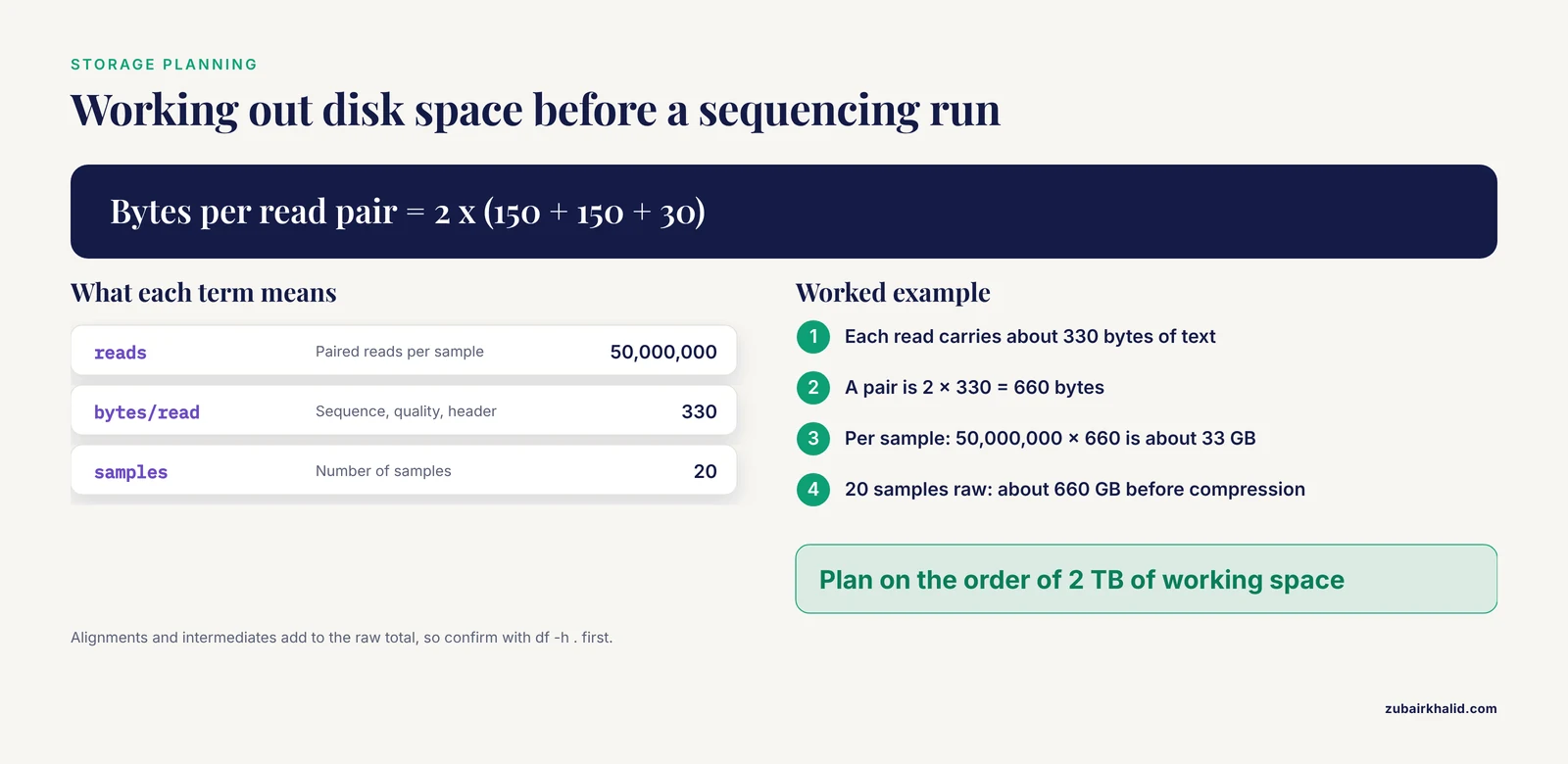
A worked calculation shows why planning matters. For one sample with 50 million paired reads of 150 bases each, each FASTQ record carries roughly 150 sequence characters, 150 quality characters, and about 30 characters of header and line breaks, about 330 bytes per read.
Bytes per read pair ≈ 2 × 330 = 660 bytes
Per sample          ≈ 50,000,000 × 660 ≈ 33 GB (before compression)
20 samples raw      ≈ 660 GB
Alignment typically produces BAM files of comparable or larger size, plus intermediate files. A project of this size needs on the order of 2 TB of working space. Confirm with df -h . before launching, not after.
Step 6: Run a versioned workflow on the small scale
Write the workflow as code in a Snakefile at the project root:
SAMPLES = glob_wildcards("data/raw/{sample}_R1.fastq.gz").sample

rule all:
    input:
        "results/multiqc/multiqc_report.html"

rule fastqc:
    input:
        "data/raw/{sample}_R1.fastq.gz",
        "data/raw/{sample}_R2.fastq.gz"
    output:
        "results/fastqc/{sample}_R1_fastqc.html",
        "results/fastqc/{sample}_R1_fastqc.zip",
        "results/fastqc/{sample}_R2_fastqc.html",
        "results/fastqc/{sample}_R2_fastqc.zip"
    shell:
        "fastqc -o results/fastqc -t 2 {input}"

rule multiqc:
    input:
        expand("results/fastqc/{sample}_R1_fastqc.zip", sample=SAMPLES),
        expand("results/fastqc/{sample}_R2_fastqc.zip", sample=SAMPLES)
    output:
        "results/multiqc/multiqc_report.html"
    shell:
        "multiqc -f -o results/multiqc results/fastqc"
Execute it:
mkdir -p results/fastqc results/multiqc
snakemake -c 8
Expected output:
Building DAG of jobs...
Job stats:
job       count
-------   -----
all           1
fastqc        4
multiqc       1
total         6
...
Finished job 0.
100% of 1 steps (6/6) done
Complete log: .snakemake/log/2026-11-11T091512.snakemake.log
The -c 8 flag requests eight cores. Because the workflow is code in Git, rerunning after an edit rebuilds only what changed, which is the core value a workflow engine adds over a shell script.
Step 7: Scale up with a community pipeline
When you move from QC to alignment, quantification, and differential expression, use a maintained pipeline. Put parameters in config/nextflow.config rather than on the command line:
params {
  input  = 'data/metadata/samplesheet.csv'
  outdir = 'results/pipeline'
}
Then run:
nextflow run nf-core/rnaseq -profile docker -resume -ansi falseExpected output looks like this:
Launching `nf-core/rnaseq` [gloomy_babbage] DSL2 - revision: (local)
[-        ] NFCORE_RNASEQ:RNASEQ:INPUT_CHECK:SAMPLESHEET_CHECK |
...
Completed at 09-Nov-2026 11:42:07
Duration    : 2h 14m
The -profile docker flag runs each step in its own container, which pins tool versions independently of your Conda environment. The -resume flag caches completed steps, so a corrected sample sheet triggers recomputation of only the affected samples. BILBO takes this consolidation further, automating retrieval of public or private RNA-seq data through the full interpretation stage in a single containerized environment [3], and it is a reasonable model for what a mature internal platform looks like.
Step 8: Aggregate quality control
MultiQC collects per-sample reports into one cross-sample document:
multiqc -f -o results/multiqc results/pipeline/pipeline_infoExpected console output:
Analysis complete for 8 tools
Report written to results/multiqc/multiqc_report.html
The report lets you spot one failed library among dozens without opening individual files.
Step 9: Verify that the result is right
Verification is a habit, not an afterthought. For an alignment output, check read statistics directly:
samtools flagstat results/pipeline/star/WT_rep1/WT_rep1.sorted.bamExpected output (counts vary with your data):
49321482 + 0 in total (QC-passed reads + QC-failed reads)
...
91.44% of reads have a paired mate that mapped
Three checks catch most problems: total read counts should match the expected library size, the percentage of uniquely mapped reads should be consistent across samples within a condition, and sample names in output tables should match the sample sheet exactly. If a number is wildly off, suspect the sample sheet first.
Step 10: Capture provenance
Record what ran, when, and with what code:
git add Snakefile config/ results/multiqc/multiqc_report.html
git commit -m "RNA-seq QC pass, 4 samples, snakemake v9"
nextflow log > logs/nextflow_history.txt
Provenance is the layer that connects a result back to the samples, references, and decisions that produced it. A structured review of agentic AI systems in bioinformatics found that published platforms implement safeguards such as sandboxed execution, interaction logs, evidence identifiers, and automated checks, yet reports rarely provide a connected account linking the original biological question to samples, reference resources, analytical decisions, and validated results [4]. Human-run projects suffer the same gap when provenance is optional, so treat the log files and commit history as deliverables, not byproducts.
Metadata That Machines Can Read
Metadata failures are silent. A count matrix with columns named 1, 2, 3 is unusable, while one with columns WT_rep1 through KO_rep2 links directly to a design table. Three practices fix this:
- Keep one master sample sheet with columns for sample ID, condition, batch, sequencing lane, and file paths, and derive every analysis input from it.
- Use community metadata standards where they exist. For microarray and sequencing experiments, the MIAME and MINSEQE families of standards define the minimum information a repository expects, which is also the minimum your future self needs.
- Store metadata in plain text (CSV or YAML) next to the data, not in a spreadsheet only one person can open.
The payoff shows up when you reuse public data. One integrative study downloaded a public keratoconus corneal RNA-sequencing dataset (GEO accession GSE77938) with separate discovery and replication cohorts, reanalyzed it with DESeq2 to define a replicated differentially expressed gene set, and then integrated that organized result with disease-gene evidence from the Open Targets Platform and extracellular-vesicle cargo from ExoCarta and Vesiclepedia to compute a transparent Cargo Prioritization Score [5]. That chain of reuse only worked because the original data carried usable cohort structure. On the systems side, CCCView demonstrates the same principle at scale, applying a unified cell-type annotation workflow across 699 spatial transcriptomics samples and over 7.4 million inferred cell-cell communication interactions so that results from heterogeneous studies become searchable and comparable [6].
Organizing High-Dimensional Data
Sequencing and microarray platforms produce matrices with tens of thousands of features measured on tens or hundreds of samples. Organization here is not only about files, it is about representing the data at the right dimensionality for each task.
Feature selection removes variables that add noise rather than signal. In clinical prediction settings, many measured identifiers are uninformative or even harmful to a decision-support model, and removing them shortens model training time and improves decision quality [1]. Dimensionality reduction complements it by projecting thousands of correlated features into a few components. The Improved Singular Value Decomposition (ISVD) approach is one such method, used after feature selection to compress large microarray data while retaining the structure needed by a downstream classifier [1]. A singular value decomposition factors a matrix of samples by features into orthogonal components ordered by the variance they explain, which lets you keep, for example, the top components that capture most of the variance and discard the rest.
The organizational implication is concrete. Keep the full raw matrix in your processed-data layer, then store reduced representations (principal component scores, selected feature lists, model inputs) as separate, named artifacts. Never overwrite the full matrix with a reduced one, because the reduction is a modeling decision that may change.
Data Organization for Spatial Transcriptomics
Spatial transcriptomics adds a coordinate system to gene expression, and the field shows how platform design shapes data organization in real time.
Serval is a modular framework for decoding imaging-based spatial transcriptomics data that separates key decoding stages into independently configurable modules, so alternative algorithms can be swapped into one position without rewriting the rest of the pipeline [7]. Its developers showed the framework generalizes across platforms by extending from MERFISH to DART-FISH [7]. That modularity is a data-organization decision, it defines stable interfaces between pipeline stages so that data flowing between them stays comparable.
Downstream stages raise the same need. OT-knn aligns spatial transcriptomics datasets across tissue sections, individuals, platforms, and developmental stages by reconstructing each spot from its spatial k-nearest neighbors inside an optimal transport framework, which makes alignment robust to sparse expression and geometric distortion between slices [8]. Alignment, like decoding, only works when data from different sources share a coherent spatial and molecular representation.
Benchmarking efforts make the organizational stakes measurable. A benchmark of 11 segmentation methods across 15 datasets from 5 spatial transcriptomics technologies found substantial variation in performance and showed that the choice of segmentation method critically shapes downstream analyses including cell-type specificity and ligand-receptor inference, and the authors released a unified Nextflow pipeline as a scalable, standardized foundation for evaluation [9]. For anyone building a spatial platform, the lesson is to record which segmentation method produced each cell-by-gene matrix, because the matrix inherits that choice.
Other fields are codifying organization in the same way. A study of antimicrobial resistance in 20,296 bacterial genomes formalized a 16-step genomic annotation protocol integrating promoter strength, mobile element context, and chromosomal point mutations, then benchmarked classifiers on the organized result [10]. A written, numbered protocol is one of the simplest and most durable forms of data organization.
Data Organization in Proteomics Platforms
Proteomics platforms face the same structure with different file types, and recent controlled work shows how much organizational choices matter.
In data-independent acquisition (DIA) proteomics, controlled quantitative experiments using defined mixtures of human, yeast, and bacterial proteomes on two mass spectrometry platforms identified over 10,000 unique proteins and over 160,000 precursors with strong accuracy and precision, and found that postprocessing options in the DIA-NN analysis stack had drastic impacts on identification rates, quantitative precision, and the false quantitative rate, in one optimal configuration reducing the false quantitative rate from roughly 0.1 to 0 with minimal identification losses [11]. The practical point for data organization is that postprocessing settings are data-shaping decisions and must be recorded per dataset, because two organizations of the same spectra can yield different protein tables.
Downstream, harmonization is an organizational problem across tools. A benchmark of seven publicly available search engines across four datasets and multiple mass spectrometry platforms showed that peptide-spectrum match rescoring substantially increased identification consensus and reduced variability between engines, although prediction-based rescoring showed a tendency toward false discovery rate underestimation in specific configurations [12]. When your platform routes data through different search engines, storing the rescoring method alongside the identification table is what makes cross-engine results comparable.
Cross-technology comparison raises the bar again. A review of circulating proteomic markers for multicancer early detection organized candidate proteins across Olink, SomaScan, and mass spectrometry evidence into biologically coherent modules on a shared axis, demonstrating that platform-level organization can make heterogeneous assay outputs interpretable together [13].
Comparing Platforms: A Practical Framework
A bioinformatics tools comparison is only useful when the categories being compared are clear. Use this table as the framework.
| Platform category | What it organizes | Strength | Watch for | Example in the literature |
|---|---|---|---|---|
| Workflow engine (Snakemake, Nextflow) | Your own pipeline steps, dependencies, caching | Full control, resumable, versionable | You must maintain metadata and environments yourself | Unified segmentation benchmark pipeline [9] |
| Self-hosted containerized platform | The full path from data acquisition to interpretation | End-to-end consistency on your own hardware | Setup and maintenance burden | BILBO [3] |
| Curated database | Preprocessed reference data | Expert curation, stable identifiers | Coverage may lag new assays | Cancer-focused databases [2] |
| Analytical web server | One analysis at a time in a browser | No installation, guided use | Limited customization, upload size limits | Cancer web servers [2] |
| Integrated analysis platform | Databases, tools, and analysis in one place | Broad capability under one interface | Complexity, learning curve | Cancer platforms [2] |
| Knowledge platform with precomputed results | Annotated, searchable results across studies | Cross-sample exploration at scale | You inherit the platform's processing choices | CCCView [6] |
| Agentic AI system | Tool selection, code execution, iterative analysis | Accelerates pipeline assembly and revision | Delegated decisions need oversight and traceability | Reviewed agentic systems [4] |
When someone asks for the best bioinformatics software, the honest answer is that the best choice is the category that matches the question, then the best-maintained tool inside that category. The review framework for cancer resources evaluates candidates by data coverage, analytical capability, evidence strength, and appropriate use case [2], and that same evaluation logic works for any domain.
Reusing Public Data Without Chaos
Public repositories are the largest storage layer in the field, and organized reuse of them is a competitive advantage. A disciplined pattern:
- Record the accession (for example GSE77938) in your sample sheet alongside your own samples, so public and local data live in one organized table.
- Download into
data/rawunder a subdirectory named for the accession, and checksum it on arrival like any local file. - Document the original processing in
references/, because public datasets carry the organizational decisions of the original authors.
The keratoconus study cited above is the model, it reanalyzed a public GEO dataset with clearly separated discovery and replication cohorts, then layered on curated external resources including STRING for protein-protein interactions and Open Targets for disease-gene evidence, all connected by an explicit scoring scheme [5]. Every link in that chain is an organizational act.
Common Mistakes and Limitations
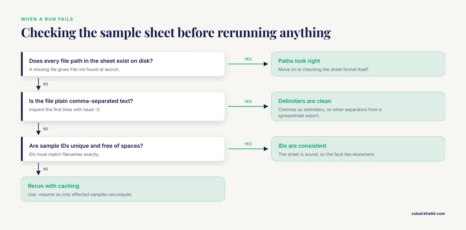
These are the failures seen most often in real projects, each with its fix.
- Editing raw files. Trimming adapters by overwriting FASTQ files destroys the anchor of reproducibility. Fix, raw data is read-only, all transformations write to
results/. - Skipping checksums. Silent truncation during file transfer is common. Fix, run
md5sum -cbefore analysis and after every transfer. - Sample sheet drift. A sample renamed in the sheet but not on disk produces errors like
File not found: data/raw/WT_rep1_R1.fastq.gz. Fix, generate filenames from the sample sheet, never the reverse, and validate the sheet before launching. - Delimiter corruption from spreadsheets. Exporting a CSV from Excel with semicolon separators causes parse failures at line 2 of the sample sheet. Fix, always export plain comma-separated text and inspect it with
head -2. - Mixing raw and processed data. Once a count matrix sits in
data/raw, no one trusts anything. Fix, the four-layer layout from earlier in this article, enforced with directory permissions where possible. - Rerunning without caching. Full recomputation after a one-line fix wastes hours to days. Fix, use
-resumein Nextflow or Snakemake's incremental execution. - Treating default postprocessing as neutral. In DIA proteomics, postprocessing choices measurably change identification and error rates, so defaults are decisions [11]. Fix, record and report them.
- Over-trusting automated agents. Agentic systems that select tools and execute code redistribute decisions that determine whether conclusions are valid, and published reports rarely connect decisions to evidence end to end [4]. Fix, review delegated analytical decisions the way you would review a student's analysis.
- Ignoring processing-choice provenance. Segmentation method choice shapes downstream cell-type and interaction results in spatial transcriptomics [9], and rescoring strategy shapes identification across search engines in proteomics [12]. Fix, store the method identifier with every derived matrix.
- Unbounded storage assumptions. The worked budget above shows a 20-sample project can exceed 2 TB. Fix, budget before running, clean intermediates on schedule, and compress with CRAM where reference-based compression applies.
One limitation belongs in its own sentence. Any individual analysis, particularly one feeding clinical interpretation, needs domain-specific statistical and subject-matter review, and no organizational scheme substitutes for expert judgment of the biology.
Practical Tips
- Write the sample sheet before downloading data, because it forces decisions about identifiers early.
- Name files with the sample ID and a processing-stage suffix, for example
WT_rep1_R1.fastq.gzandWT_rep1.sorted.bam, so a sorted listing tells the project's story. - Commit configuration files to Git at the same moment you change them, not at the end of the project.
- Prefer plain-text formats (CSV, YAML, VCF) for anything a human may need to read under time pressure, and binary formats (CRAM, HDF5) for anything large that software reads.
- Run one end-to-end test on a single sample before launching a full cohort, which catches sample-sheet and path errors in minutes instead of hours.
- Keep a project-level
README.mdrecording what each directory contains, updated when the layout changes. - When evaluating a new tool for your platform, run it on a small controlled dataset with known expected results before trusting it on real data, mirroring the controlled-experiment logic used in quantitative proteomics [11].
Frequently Asked Questions
What is data organization in bioinformatics platforms?
It is the practice of arranging raw data, metadata, processed results, and code into stable, separable layers so that any analysis can be verified and rerun. On real platforms this means immutable raw files, machine-readable sample sheets, regenerable outputs, and versioned workflows [3].
How do I organize a bioinformatics project step by step?
Create a fixed directory skeleton, pin the software environment with Conda, checksum the raw data, build a single sample sheet, run a workflow engine, aggregate quality control, and commit configuration and logs to Git. The ten-step walkthrough earlier in this article gives the exact commands and expected outputs.
What is the best bioinformatics software for managing workflows?
There is no single best tool, the best choice depends on category and use case. For pipeline management, Snakemake and Nextflow are the established workflow engines, and for full end-to-end needs a containerized platform such as BILBO or a curated resource selected with a coverage-and-use-case framework may serve better [3][2].
Which file formats should I use for genomics and proteomics data?
Use community-standard formats, FASTQ for raw reads, BAM or CRAM for alignments, VCF for variants, and HDF5 or Zarr-backed containers such as AnnData for large matrices and single-cell objects. Standard formats carry indexes, documentation, and tool support that ad hoc formats lack.
How much storage does a typical sequencing project need?
Budget roughly 33 GB of raw FASTQ per sample for 50 million paired 150-base reads before compression, and plan for two to three times that total once alignments and intermediates are included. The worked calculation earlier in this article shows the arithmetic to adapt to your own read counts.
How do I keep raw data safe from accidental edits?
Checksum raw files on arrival with md5sum, store the checksum table in metadata, store raw files in a write-protected directory, and verify with md5sum -c after every transfer. Any FAILED line means the file must be replaced before analysis.
What are the most common mistakes in bioinformatics data organization?
The most common are editing raw files, skipping checksums, letting sample sheets drift out of sync with filenames, mixing raw and processed data, and failing to record processing choices such as postprocessing and segmentation settings that measurably shape results [11][9]. Each has a concrete fix listed in the mistakes section above.
How do I make my bioinformatics analysis reproducible?
Combine four elements, immutable raw data with checksums, a pinned environment (Conda export or containers), a versioned workflow engine run, and captured provenance linking samples, references, decisions, and outputs. Current reviews emphasize that this connected provenance chain, not just tool availability, is what makes conclusions trustworthy [4].
Sources
- Optimized Attribute Selection Using Artificial Plant (AP) Algorithm with ESVM Classifier (AP-ESVM) and Improved Singular Value Decomposition (ISVD)-Based Dimensionality Reduction for Large Micro-array Biological Data.
- Web servers and bioinformatics tools for cancer research: A review.
- BILBO: a self-hosted platform for large-scale RNA-Seq analysis with a functional annotation clustering framework.
- Trustworthy Agentic AI in Bioinformatics: From Workflow Automation to Traceable and Validated Biological Inference.
- An Integrative Bioinformatics Framework Nominates Candidate Limbal Stem-Cell Exosome Cargo for Keratoconus by Coupling Corneal Transcriptomics, Disease-Gene Evidence and Extracellular-Vesicle Repositories.
- CCCView: A Knowledge Platform for Integrated Analysis of Spatial Transcriptomic Cell-Cell Communication.
- Serval: a modular framework for decoding imaging based spatial transcriptomics data.
- OT-knn: A neighborhood-aware optimal transport framework for aligning spatial transcriptomics data.
- Benchmarking segmentation methods for spatial transcriptomics.
- Uncovering species- and drug-class-specific antimicrobial resistance mechanisms from large-scale whole-genome sequencing data using discordance analysis and machine learning.
- Recommendations for Quantitative Data-Independent Acquisition (DIA) Proteomics Using Controlled Quantitative Experiments (CQEs).
- From Variability to Consensus: Rescoring Harmonizes Peptide Identification across Diverse Search Engines and Data Sets.
- Circulating Proteomic Signatures for Multicancer Early Detection: Cross-Platform Evidence for a Matrix-Immune-Secretory Biomarker Axis.