How to Create a SummarizedExperiment Object from Scratch
By Dr. Zubair Khalid, DVM, MS, PhD ·

By the end of this guide you will be able to create a SummarizedExperiment object from scratch in R, starting from nothing more than a count matrix, a sample sheet, and an annotation table. You will attach a second assay, compute sample-level statistics, keep rows and columns synchronized while subsetting, validate the result, and save the finished object for downstream analysis.
Here is what to have ready. Install R 4.4 or newer, then install Bioconductor and the SummarizedExperiment package. On the data side, bring a features-by-samples matrix (a CSV export from a quantification pipeline is typical), a sample metadata table with one row per sample, and optionally a feature annotation table or genomic coordinates.
The SummarizedExperiment class is an S4 class (R's system for formal object classes with defined slots) and it is Bioconductor's standard container for matrix-shaped genomics data. It stores one or more matrix-like assays together with metadata for the rows (features) and the columns (samples) inside a single validated object [1]. If you are learning R for bioinformatics, this object is the handoff point between quantification and statistics. Bioconductor covers the full path, from raw read input and quality assessment with packages such as ShortRead [2] to analysis and visualization layers such as exvar [3], and most quantified outputs land in a SummarizedExperiment at some point in a workflow.
Why This Container Is the Standard in R for Bioinformatics
Three properties explain the adoption. First, synchronization. The assay matrix, the feature metadata, and the sample metadata travel together, so any row or column subset keeps all three aligned. Second, validation. The constructor refuses objects with mismatched dimensions or inconsistent names, which catches the most common data handling mistakes at build time rather than mid-analysis. Third, interoperability. Downstream packages are written against this interface, so a well-formed object plugs directly into normalization, differential expression, and visualization tools.
The interoperability argument is easy to demonstrate. The slinky package, which streamlines access to the LINCS L1000 perturbation dataset, encapsulates its expression data as a SummarizedExperiment object precisely so the data integrates with Bioconductor workflows [4].
The container also anchors a broader design pattern. Bioconductor packages frequently define purpose-built containers that reuse shared conventions: GenomicInteractions for chromatin interaction data from Hi-C and related assays [5], InteractionSet, which supplies base classes for genomic interactions and builds on existing Bioconductor infrastructure [6], QTLExperiment for multi-state QTL summary statistics, built on existing Bioconductor infrastructure and conventions [7], and tidyCoverage, whose CoverageExperiment and AggregatedCoverage classes extend the SummarizedExperiment class directly [8]. Once you can build a plain SummarizedExperiment, you can read, construct, and extend all of these specialized containers, because they expose the same assay, rowData, and colData interface.
The Format: Four Slots You Fill
A SummarizedExperiment holds four things. The assays slot stores one or more matrices with features as rows and samples as columns (an assay is simply one such measurement matrix, for example raw counts or normalized expression). The rowData slot stores a DataFrame, an S4 table class from the S4Vectors package that keeps row names stable and allows list-valued columns, with exactly one row per feature. The colData slot stores a DataFrame with exactly one row per sample. The metadata slot stores a named list for experiment-wide notes such as genome build or processing version. Optionally, genomic coordinates for the features go into the rowRanges slot as a GRanges object, an interval container with chromosome, start, end, and strand from the GenomicRanges package. Features can be genes, transcripts, proteins, CpG sites, or genomic bins depending on the assay.
| Slot | Constructor argument | Accessor | Required type | Rule it enforces |
|---|---|---|---|---|
| , - | , - | , - | , - | , - |
| assays | assays = | assay(), assays(), assayNames() | matrix-like objects in a named list | all assays share the same dimensions |
| rowData | rowData = | rowData() | DataFrame (or GRanges, see below) | nrow equals the assay nrow |
| rowRanges | pass a GRanges as rowData = | rowRanges() | GRanges or GRangesList | length equals the assay nrow |
| colData | colData = | colData() | DataFrame | nrow equals the assay ncol |
| metadata | metadata = | metadata() | named list | no constraint |
Two rules govern construction. Every assay must have the same dimensions, and the number of rowData rows must equal the number of assay rows while the number of colData rows must equal the number of assay columns. Row and column names must either be absent from the assay or match the rowData and colData names exactly.
Reading the printed format
Print the object and R summarizes the whole structure in a few lines:
seclass: SummarizedExperiment
dim: 6 4
metadata(2): experiment genome
assays(1): counts
rownames(6): ENSG00000001 ENSG00000002 ... ENSG00000006
rowData names(2): gene_name gene_biotype
colnames(4): S1 S2 S3 S4
colData names(2): condition batchRead it line by line. dim gives features by samples. The assays line lists assay names in order. The rownames line shows feature identifiers, which come from the rowData row names. The colnames line shows sample identifiers from colData. The last two lines list the metadata columns available on each axis. Whenever you receive an object from a collaborator or a package, this printout plus validObject() is the fastest structural audit.
What You Need Installed
Bioconductor releases are paired with R versions, and current releases require R 4.4 or newer. Install the manager from CRAN, then install the package:
install.packages("BiocManager")
BiocManager::install("SummarizedExperiment")
For the later sections on sparse and file-backed assays, install two more packages:
BiocManager::install(c("Matrix", "HDF5Array", "GenomicRanges"))Confirm the setup:
library(SummarizedExperiment)
packageVersion("SummarizedExperiment")
BiocManager::version()
Worked Example: Create a SummarizedExperiment Object from Scratch
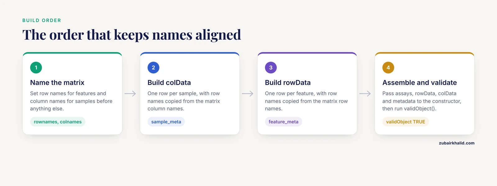
This walkthrough builds a small synthetic RNA-seq object with 6 genes and 4 samples, then extends and subsets it. Every block is self-contained, so you can paste them in order.
Step 1: Load the package
library(SummarizedExperiment)Step 2: Build the assay matrix
The assay must be a matrix with row names for features and column names for samples. Name both dimensions now, because names are what let the constructor verify alignment later.
counts <- matrix(
  c(120, 45, 300, 8, 950, 12,
    135, 52, 280, 11, 1010, 9,
    60, 48, 295, 10, 990, 15,
    66, 41, 310, 7, 940, 11),
  nrow = 6, ncol = 4
)
rownames(counts) <- sprintf("ENSG%08d", 1:6)
colnames(counts) <- paste0("S", 1:4)
counts
S1 S2 S3 S4
ENSG00000001 120 135 60 66
ENSG00000002 45 52 48 41
ENSG00000003 300 280 295 310
ENSG00000004 8 11 10 7
ENSG00000005 950 1010 990 940
ENSG00000006 12 9 15 11Step 3: Build colData (sample metadata)
Use DataFrame(), not data.frame(), and assign row names that match the matrix column names exactly.
library(S4Vectors)
sample_meta <- DataFrame(
  condition = factor(c("control", "control", "treated", "treated")),
  batch = factor(c("b1", "b2", "b1", "b2"))
)
rownames(sample_meta) <- colnames(counts)
sample_meta
DataFrame with 4 rows and 2 columns
condition batch
<factor> <factor>
S1 control b1
S2 control b2
S3 treated b1
S4 treated b2Step 4: Build rowData (feature metadata)
Same pattern on the feature axis.
feature_meta <- DataFrame(
  gene_name = paste0("GENE", 1:6),
  gene_biotype = rep("protein_coding", 6)
)
rownames(feature_meta) <- rownames(counts)
Step 5: Assemble the object
se <- SummarizedExperiment(
  assays = list(counts = counts),
  rowData = feature_meta,
  colData = sample_meta,
  metadata = list(
    experiment = "synthetic pilot RNA-seq",
    genome = "GRCh38"
  )
)
se
The printed object matches the format shown earlier. If any dimension or name is off, the constructor fails here with a validation error rather than producing a broken object.
Step 6: Inspect the object
dim(se)            # 6 4
assayNames(se)     # "counts"
head(assay(se, "counts"))
colData(se)
rowData(se)
metadata(se)
Three accessors cover daily work. assay(se, "counts") returns one assay, assay(se) returns the first one, and se[["counts"]] is shorthand for the same thing. The $ operator reads colData columns, so se$condition returns the condition factor.
Step 7: Add a second assay and sample statistics
Assay assignment requires the new matrix to have exactly the dimensions of the object. A log transform is the classic example:
assay(se, "logcounts") <- log2(assay(se, "counts") + 1)
assayNames(se)
# [5] "counts"    "logcounts"
Sample-level statistics belong in colData. Here the library size (the total read count per sample) is computed and attached:
colData(se)$library_size <- colSums(assay(se, "counts"))
colData(se)
DataFrame with 4 rows and 3 columns
condition batch library_size
<factor> <factor> <numeric>
S1 control b1 1435
S2 control b2 1497
S3 treated b1 1418
S4 treated b2 1375Step 8: Add genomic coordinates (optional)
Pass a GRanges as the rowData argument and the constructor stores the intervals in rowRanges while its metadata columns become rowData:
library(GenomicRanges)
gr <- GRanges(
  seqnames = rep("chr17", 6),
  ranges = IRanges(start = seq(1000, 6000, by = 1000), width = 1200),
  strand = "+",
  gene_name = feature_meta$gene_name,
  gene_biotype = feature_meta$gene_biotype
)
names(gr) <- rownames(feature_meta)

se_gr <- SummarizedExperiment(
  assays = list(counts = counts),
  rowData = gr,
  colData = sample_meta
)
rowRanges(se_gr)   # the GRanges with coordinates
rowData(se_gr)     # the metadata columns gene_name and gene_biotype
Step 9: Subset without losing metadata
Subsetting uses matrix-like indexing, and the metadata follows automatically:
se_treated <- se[, se$condition == "treated"]
dim(se_treated)
# [5] 6 2
assay(se_treated, "counts")
S3 S4
ENSG00000001 60 66
ENSG00000002 48 41
ENSG00000003 295 310
ENSG00000004 10 7
ENSG00000005 990 940
ENSG00000006 15 11Row subsetting works the same way:
se_small <- se[1:3, 1:2]
dim(se_small)
# [5] 3 2
One caveat matters for very large data. Each subset is a new object holding a copy of the assay, which costs memory and breaks the link back to the parent object. This exact limitation motivated the ExperimentSubset package, which stores subsets inside the parent container while preserving provenance [1].
Step 10: Save and reload
saveRDS(se, "pilot_se.rds")
se_reloaded <- readRDS("pilot_se.rds")
identical(assay(se_reloaded, "counts"), assay(se, "counts"))
# [5] TRUE
A Reusable Template for Your Own Data
The following function is a create summarizedexperiment object template you can drop into a project. It takes a counts table, a sample sheet, and a feature table, enforces the naming rules, and returns a validated object.
make_se <- function(counts, samples, features,
                    sample_id = "sample_id", feature_id = "gene_id",
                    experiment_name = "untitled experiment") {
  counts <- as.matrix(counts)
  storage.mode(counts) <- "numeric"

  samples <- as(samples, "DataFrame")
  features <- as(features, "DataFrame")

  stopifnot(sample_id %in% colnames(samples))
  stopifnot(feature_id %in% colnames(features))

  rownames(samples) <- samples[[sample_id]]
  samples[[sample_id]] <- NULL
  rownames(features) <- features[[feature_id]]
  features[[feature_id]] <- NULL

  if (anyDuplicated(rownames(features)) > 0) {
    stop("duplicated feature ids in the annotation table")
  }
  if (!identical(colnames(counts), rownames(samples))) {
    stop("sample names in the count matrix and sample sheet do not match")
  }
  if (!identical(rownames(counts), rownames(features))) {
    stop("feature names in the count matrix and annotation table do not match")
  }

  SummarizedExperiment(
    assays = list(counts = counts),
    rowData = features,
    colData = samples,
    metadata = list(experiment = experiment_name)
  )
}
Usage with data frames already loaded in R:
se_new <- make_se(
  counts = counts_df,
  samples = sample_sheet,
  features = gene_table,
  experiment_name = "pilot RNA-seq"
)
The three stop() checks turn silent misalignment into loud failures. Keep them, even when you are in a hurry, because they catch the errors that are hardest to notice later.
Loading Real Data from CSV Files
Three files cover most bulk experiments: a counts CSV with feature identifiers in the first column, a samples CSV, and a genes CSV.
counts_raw <- read.csv("counts.csv", row.names = 1, check.names = FALSE)
counts <- as.matrix(counts_raw)
storage.mode(counts) <- "numeric"

samples <- read.csv("samples.csv")
if (anyNA(match(colnames(counts), samples$sample_id))) {
  stop("some samples in the count matrix are missing from the sample sheet")
}
samples <- samples[match(colnames(counts), samples$sample_id), ]
rownames(samples) <- samples$sample_id
samples$sample_id <- NULL

genes <- read.csv("genes.csv")
rownames(genes) <- genes$gene_id
genes$gene_id <- NULL

stopifnot(identical(rownames(counts), rownames(genes)))

se <- SummarizedExperiment(
  assays = list(counts = counts),
  rowData = genes,
  colData = samples
)
Two arguments do heavy lifting here. row.names = 1 moves feature identifiers out of the data frame and into row names. check.names = FALSE preserves sample identifiers exactly as written, which matters because the default check.names = TRUE rewrites names that start with a digit (a sample called 1 becomes X1), and that rewrite then triggers a name mismatch at construction.
If your annotation table is ordered differently from the count matrix, the match() line reorders it correctly. Never rely on both files happening to be sorted the same way.
Choosing the Assay Representation: Dense, Sparse, or File-Backed
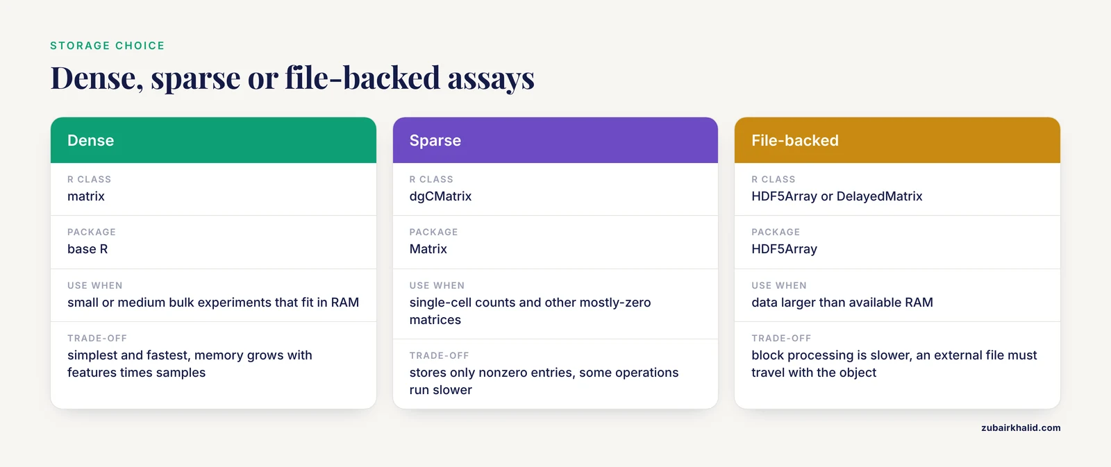
The assays slot accepts any matrix-like object, which lets you match the representation to the data size.
| Representation | R class | Package | Use when | Trade-off |
|---|---|---|---|---|
| , - | , - | , - | , - | , - |
| Dense | matrix | base R | small or medium bulk experiments that fit in RAM | simplest and fastest, memory grows with features times samples |
| Sparse | dgCMatrix | Matrix | single-cell counts and other mostly-zero matrices | stores only nonzero entries, some operations run slower |
| File-backed | HDF5Array or DelayedMatrix | HDF5Array | data larger than available RAM | near-unlimited size, block processing is slower, an external file must travel with the object |
Sparse storage is the standard for single-cell data, where most entries are zero. The beachmat project was built on this observation, noting that large single-cell matrices require sparse or file-backed representations for memory-efficient handling in R, and it defines a clear memory and speed trade-off to guide the choice of representation [9].
library(Matrix)
counts_sparse <- as(counts, "dgCMatrix")
se_sparse <- SummarizedExperiment(
  assays = list(counts = counts_sparse),
  rowData = feature_meta,
  colData = sample_meta
)
class(assay(se_sparse, "counts"))
# [5] "dgCMatrix"
For data that exceeds RAM, write the assay to an HDF5 file and wrap it. A DelayedArray is a matrix-like wrapper that keeps data on disk and computes in blocks on demand:
library(HDF5Array)
counts_h5 <- writeHDF5Array(counts, filepath = "assays.h5", name = "counts")
se_h5 <- SummarizedExperiment(
  assays = list(counts = counts_h5),
  rowData = feature_meta,
  colData = sample_meta
)
as.matrix(assay(se_h5, "counts")[1:2, 1:2])
S1 S2
ENSG00000001 120 135
ENSG00000002 45 52On-disk representations have precedent across Bioconductor. MSnbase introduced on-disk infrastructure so that large raw mass spectrometry experiments can be handled on commodity hardware [10], and the same principle underlies file-backed assays in genomics containers.
Validating the Object Before Analysis
Run four checks on every object you build or receive. validObject() runs the full structural validation and returns TRUE when the object passes:
validObject(se)
# [5] TRUE
Then verify that the names on both axes are exactly what you expect, that no values are missing, and that no sample has a zero or negative total:
stopifnot(identical(colnames(se), rownames(colData(se))))
stopifnot(identical(rownames(se), rownames(rowData(se))))
sum(is.na(assay(se, "counts")))
# [5] 0
all(colSums(assay(se, "counts")) > 0)
# [5] TRUE
A useful final check is a round trip. Extract the assay, compare it with your original matrix, and confirm the object did not reorder anything:
identical(assay(se, "counts"), counts)
# [5] TRUE
Common Errors, Exact Messages, and Fixes
| Message fragment | Trigger | Fix |
|---|---|---|
| , - | , - | , - |
could not find function "SummarizedExperiment" | package not installed or not attached | BiocManager::install("SummarizedExperiment") then library(SummarizedExperiment) |
'colData' nrow must equal the assay ncol | sample metadata rows differ from matrix columns | match counts, then reorder with samples[match(colnames(counts), samples$sample_id), ] |
'rowData' nrow must equal the assay nrow | annotation rows differ from matrix rows | same correction on the feature axis |
'assays' colnames must be NULL or equal to 'colData' rownames | sample names differ or are ordered differently | set rownames(colData) <- colnames(counts) after reordering |
rownames must be unique | duplicated feature identifiers | aggregate with rowsum() or relabel with make.unique() |
attempt to apply non-function | a variable named colData or rowData masks the accessor | rename your variable and rebuild it |
The full text of validation errors carries the prefix invalid class "SummarizedExperiment" object, and minor wording varies between package versions, so match on the quoted fragment rather than the whole string.
Two further errors deserve their own notes. When you assign a new assay with assay(se, "name") <- value and the value has different dimensions, the assignment fails with an error stating that the assays must share dimensions, so check dim(value) against dim(se) first. And when a saved object with an HDF5-backed assay is moved without its .h5 file, reading the assay fails with an error about the missing file, so always move the external file together with the RDS.
Common Mistakes and Limitations
- Naming your variables
colDataorrowData. This masks the accessor functions, and the nextcolData(se)call fails withattempt to apply non-function. Use names likesample_metaandfeature_meta. - Leaving the count matrix unnamed. If the assay has no dimnames, the constructor cannot verify alignment, and an annotation table sorted differently attaches the wrong metadata silently. Always set row names and column names on the matrix before construction.
- Building colData from
read.csv()output without assigning row names.read.csv()keeps identifiers as a regular column, so the DataFrame has automatic numeric row names that will not match your sample names. Assignrownames(samples) <- samples$sample_idexplicitly. - Using
assays(se) <- list(new)to add an assay. That replaces every existing assay. Useassay(se, "name") <- value, which adds or replaces a single named assay. - Confusing
$with assay access.se$countslooks in colData, not in assays, and returns NULL when no such column exists. Useassay(se, "counts")for assays. - Passing a data frame as an assay. Coerce with
as.matrix()first, because assay elements must be matrix-like objects. - Treating validation as a biology check. The constructor verifies dimensions, names, and types only. Mislabeled samples and swapped conditions pass
validObject()without complaint, so the biological checks stay your responsibility. - Ignoring memory limits. A dense matrix for a large single-cell experiment exhausts RAM quickly, which is exactly why sparse and file-backed representations exist and why the field evaluates the memory and speed trade-off explicitly [9].
- Assuming subsets remember their parent. Standard subsetting copies data into a new object and severs provenance, a limitation that motivated dedicated subset-aware containers [1].
Next Steps: Downstream Analysis and Related Containers
With a valid object in hand, the standard bulk RNA-seq path is differential expression with DESeq2, edgeR, or limma, each of which accepts the count matrix extracted with assay(se, "counts"). For single-cell data, convert once and reuse:
sce <- as(se, "SingleCellExperiment")SingleCellExperiment extends SummarizedExperiment with slots for dimensionality reductions, size factors, and alternative experiments, and it is the input format for most single-cell packages.
If you prefer dplyr-style manipulation, the tidyomics ecosystem bridges Bioconductor containers to tidy R verbs, demonstrated across six data frameworks and ten analysis tools in a single large-scale analysis [11]. The tidySummarizedExperiment package from that ecosystem lets you filter, mutate, and summarize an object with tidy verbs while returning a valid SummarizedExperiment.
Finally, watch for the container pattern when your data does not fit a features-by-samples matrix. QTL summary statistics live in QTLExperiment [7], chromatin interactions in InteractionSet-derived classes [6], and coverage tracks in tidyCoverage classes that extend SummarizedExperiment directly [8]. The package vignette on bioconductor.org remains the authoritative reference for the class, and the interface you practiced here transfers to all of them.
Frequently Asked Questions
Can I create a SummarizedExperiment object from a data frame?
Yes, but coerce it with as.matrix() first, because assay elements must be matrix-like objects. Set row names and column names on the matrix before passing it to the constructor.
What is the difference between rowData and rowRanges?
rowData holds the feature metadata table as a DataFrame. rowRanges holds genomic coordinates as a GRanges. Passing a GRanges as the rowData argument stores the intervals in rowRanges and its metadata columns in rowData.
Do I have to use DataFrame instead of data.frame for colData?
No, current versions coerce a plain data.frame automatically. DataFrame is still recommended because it preserves row names reliably and supports list-valued columns.
How do I add another assay to an existing object?
Use assay(se, "name") <- matrix with a matrix of the same dimensions as the object. Avoid assays(se) <- for this, because it replaces every existing assay.
How do I handle duplicated gene symbols?
Collapse or relabel them before construction, because row names must be unique. Sum counts per symbol with rowsum(counts, group = symbols) or disambiguate with make.unique(symbols).
Can I store single-cell data in a SummarizedExperiment?
Yes, typically with a sparse dgCMatrix assay. For real single-cell work use SingleCellExperiment, which extends the class with reduced dimensions and other single-cell-specific slots.
How do I save and reload a SummarizedExperiment?
Use saveRDS() and readRDS(). If an assay is file-backed with HDF5, the external .h5 file must remain at its original path or the assay cannot be read.
How is a SummarizedExperiment different from an ExpressionSet?
ExpressionSet is the older Biobase container from the microarray era. SummarizedExperiment is the current standard, with native multi-assay support, GRanges coordinates, and file-backed assay support.
Sources
- ExperimentSubset: an R package to manage subsets of Bioconductor Experiment objects.
- ShortRead: a bioconductor package for input, quality assessment and exploration of high-throughput sequence data.
- Efficient and easy gene expression and genetic variation data analysis and visualization using exvar.
- Streamlined analysis of LINCS L1000 data with the slinky package for R.
- GenomicInteractions: An R/Bioconductor package for manipulating and investigating chromatin interaction data.
- Infrastructure for genomic interactions: Bioconductor classes for Hi-C, ChIA-PET and related experiments.
- Orchestrating multi-state QTL analysis with Bioconductor.
- Epigenomics coverage data extraction and aggregation in R with tidyCoverage.
- beachmat: A Bioconductor C++ API for accessing high-throughput biological data from a variety of R matrix types.
- MSnbase, Efficient and Elegant R-Based Processing and Visualization of Raw Mass Spectrometry Data.
- The tidyomics ecosystem: enhancing omic data analyses.