How to Create a Seurat Object from Single-Cell RNA-seq Data

By Dr. Zubair Khalid, DVM, MS, PhD · 2026-11-11

By the end of this article you will be able to take raw single-cell RNA-seq count data, load it into R, and build a valid Seurat object that is ready for quality control, normalization, and clustering. You will learn the file formats that Seurat accepts, the exact commands for the three most common input types, what every important argument does, the error messages you are most likely to hit, and how to verify that the object you built actually contains what you think it contains.

To follow along you need R 4.1 or newer, the Seurat package installed from CRAN, roughly 4 to 8 GB of free RAM for a typical 10,000-cell dataset, and a count matrix from your sequencing provider. If you processed your own raw reads with CellRanger, the output folder you need is called filtered_feature_bc_matrix. If your sequencing core sent you files, look for matrix.mtx.gz, barcodes.tsv.gz, and features.tsv.gz, or a single filtered_feature_bc_matrix.h5 file.

Why the Seurat Object Exists

Single-cell RNA-seq measures gene expression in thousands of individual cells at once. Droplet-based platforms such as 10x Genomics Chromium profile thousands of cells per lane, with published protocols running roughly 20,000 cells per channel on a Chromium X instrument. The raw output of such an experiment is a sparse matrix of integer counts, one row per gene, one column per cell barcode, where the vast majority of entries are zero.

The Seurat object is a container that keeps that count matrix together with everything you compute downstream, including normalized values, dimensionality reductions, cluster labels, and per-cell metadata. Seurat is an R package maintained by the Satija Lab, and it remains the most widely used toolkit for scRNA-seq analysis in R for bioinformatics. Published workflows across immunology, oncology, and neuroscience routinely begin by loading count data into a Seurat object before clustering and annotation [3].

The same container pattern appears across the field. The Bioconductor ecosystem uses the SingleCellExperiment class for the same purpose, and packages such as Voyager build spatial analysis on top of related data structures [5]. If you plan to work in both ecosystems, it helps to understand that a Seurat object and a SingleCellExperiment object solve the same problem, and conversion between them is straightforward with packages like SeuratDisk and zellkonverter.

Understanding the Input Formats Before You Build Anything

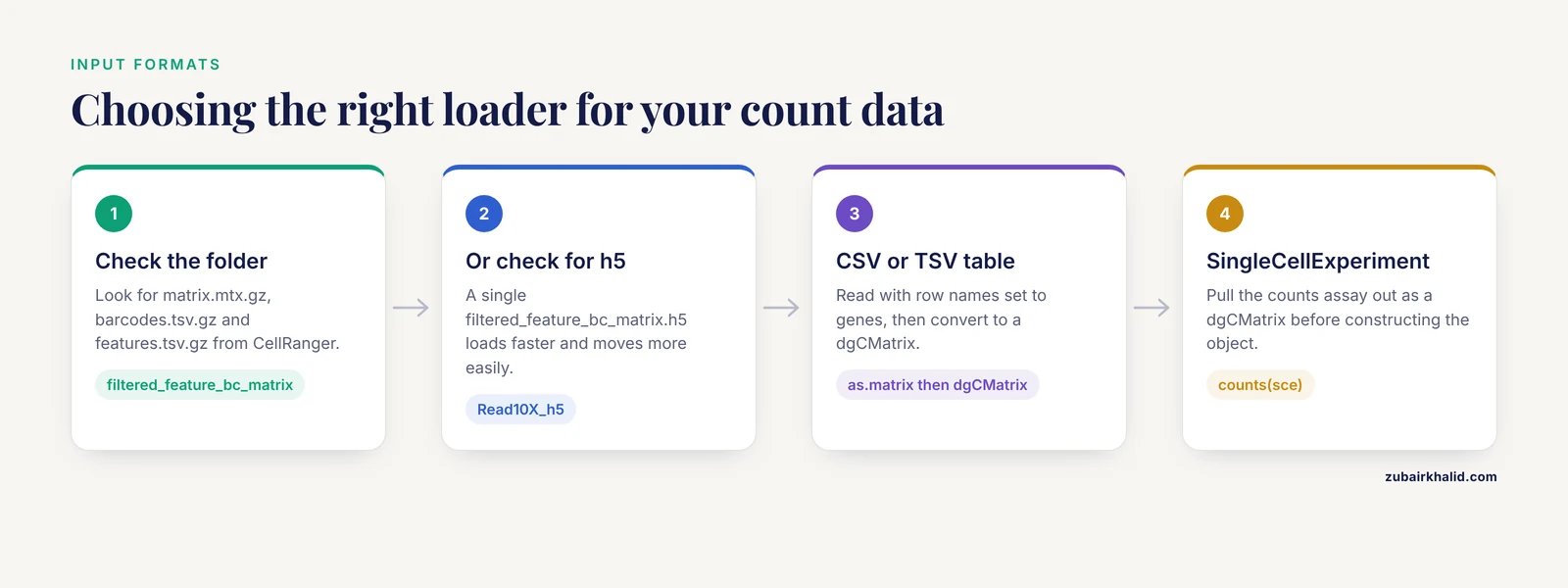
Seurat can accept count data from almost any source, but three formats cover the overwhelming majority of real projects. Recognizing the format you have is the first step in deciding which loading function to call.

The 10x Genomics three-file format (Matrix Market)

CellRanger, the 10x Genomics alignment and counting software, produces a folder with three compressed text files [1]:

• matrix.mtx.gz, a Matrix Market file holding the nonzero count entries in triplet form (row index, column index, value)
• barcodes.tsv.gz, one cell barcode per line, in the same column order as the matrix
• features.tsv.gz, one line per gene with gene ID, gene symbol, and feature type

Because droplet data is extremely sparse, this triplet representation stores only nonzero values and keeps memory use manageable. A 30,000-gene by 10,000-cell dense matrix would need billions of entries, while the actual nonzero count is usually under 10 percent of that.

The HDF5 format (.h5)

Newer CellRanger versions also write a single HDF5 file, typically filtered_feature_bc_matrix.h5. This is one binary file containing the same sparse matrix plus barcode and feature annotations. It loads faster and moves around more easily than three separate files.

A plain data frame or matrix

Public data from GEO often arrives as a gene-by-cell table in CSV, TSV, or RDS format. Published analyses describe this path directly, for example downloading scRNA-seq data from GEO and then creating a Seurat object from it in R [3]. This format is the simplest but the most memory hungry, so convert to sparse form as soon as possible.

Data you should NOT feed directly to CreateSeuratObject

Raw reads, FASTQ files, BAM files, and CellRanger report summaries are not count matrices. You must run an alignment and counting pipeline first. For standard 10x chemistry, CellRanger is the reference implementation. Specialized protocols need specialized upstream tools. For example, alternative polyadenylation measurement from 10x libraries uses a dedicated pipeline called scraps that aligns read 1 to the genome to recover polyadenylation sites [6], and full-length isoform recovery from 10x cDNA pools has been demonstrated with the R2C2 long-read approach on Oxford Nanopore data [7]. Those pipelines produce their own outputs, and only the gene-by-cell count layer belongs in a standard Seurat object.

Setting Up Your R Environment

Install R from CRAN, then install Seurat and the matrix package it depends on:

install.packages(c("Seurat", "Matrix", "Matrix.utils"))

On most systems this pulls in everything needed. Check the installation:

library(Seurat)
packageVersion("Seurat")

Expected output looks like this:

[6] '5.1.0'

Seurat 5 changed several internals relative to Seurat 4, including how layers are stored, but CreateSeuratObject behaves the same way in both. If you work across teams, agree on a Seurat major version, because saved objects from Seurat 4 can require conversion steps before Seurat 5 will touch them.

You also need a working directory with your data. Set it explicitly and confirm the files are where you think they are:

setwd("/path/to/project")
list.files("data/pbmc_filtered_feature_bc_matrix")

Expected output:

[6] "barcodes.tsv.gz" "features.tsv.gz" "matrix.mtx.gz"

Numbered Walkthrough: Building the Object from 10x Output

This walkthrough follows the canonical 10x three-file format, which is the most common create seurat object single cell rna-seq example in the literature and in tutorials [1][2].

Step 1: Read the count matrix with Read10X

library(Seurat)

counts <- Read10X(data.dir = "data/pbmc_filtered_feature_bc_matrix")

Read10X returns either a sparse matrix or, when the features file contains multiple feature types such as Gene Expression plus Antibody Capture, a named list of sparse matrices. Check what you got:

class(counts)
dim(counts)
counts[1:5, 1:5]

Expected output for a standard gene expression run:

[6] "dgCMatrix"
[6] 33538  2700

5 x 5 sparse Matrix of class "dgCMatrix"
AAACATACAACCAC-1 AAACGCTGTTCTCC-1 ...
RP11-34P13.7          .               .
RP11-34P13.11         .               .
FAM138A               .               .
OR4F5                 .               .

Two things to notice. First, the class is dgCMatrix, a compressed sparse column matrix. Second, the matrix is genes by rows and cells by columns. Seurat expects exactly that orientation. A dense matrix read from CSV with cells as rows will produce a transposed object downstream, which is one of the most common silent failures in this workflow.

Step 2: Call CreateSeuratObject

pbmc <- CreateSeuratObject(
  counts = counts,
  project = "pbmc_reference",
  min.cells = 3,
  min.features = 200,
  assay = "RNA"
)

Expected output:

Warning: Feature names cannot have underscores ('_'), replacing with dashes ('-')
An object of class seurat
33538 features across 2700 cells within 1 assay
Active assay: RNA (33538 features, 0 variable features)
1 layer present: counts

That warning about underscores appears when gene symbols contain characters Seurat treats specially. It is cosmetic in most cases, and dash replacement preserves uniqueness in practice. You now have a Seurat object. Every downstream step, from normalization to clustering, operates on it.

Step 3: Inspect what the constructor did

pbmc
head([email protected])

Expected output for the metadata:

              orig.ident nCount_RNA nFeature_RNA
AAACATACAACCAC-1 pbmc_reference       2419          779
AAACGCTGTTCTCC-1 pbmc_reference       4783         1348

Three columns are created automatically. orig.ident records the project label you supplied, nCount_RNA is the total UMI count per cell, and nFeature_RNA is the number of detected genes per cell. These two numeric columns drive your first quality control plots, so they are worth understanding now. A human PBMC cell typically has a few hundred to a few thousand detected genes, and cells far below that range are usually empty droplets or debris.

Step 4: Understand each argument that matters

The constructor filters as it builds. min.cells = 3 discards genes detected in fewer than 3 cells, which removes genes that carry no information and shrinks the matrix. min.features = 200 discards cells with fewer than 200 detected genes, which is a coarse first pass at removing empty droplets. Both thresholds are conventional starting values rather than universal rules, and you should tune them to your tissue. Published kidney dissociation protocols note that captured RNA per cell varies with tissue and protocol, which is one reason per-tissue threshold tuning matters [1].

A summary table of the arguments you will actually use:

Step 5: Add sample-level metadata

Cell-level metadata is where experimental design lives. Add it as a data frame with row names matching cell barcodes:

pbmc$condition <- "healthy"
pbmc$donor <- "D01"
head([email protected])

For multi-sample projects, build the metadata table before or right after merging, because once you lose track of which barcode came from which sample, every downstream comparison is compromised. Published cohort-scale analyses depend entirely on correct per-cell sample labels, whether they are mapping cell states across patient samples [8] or computing distances between patients from their cellular compositions [9].

Step 6: Move from raw counts to a normalized object

Creating the object is not the end of the workflow, it is the beginning. The standard first analysis pass is:

pbmc <- NormalizeData(pbmc)
pbmc <- FindVariableFeatures(pbmc, nfeatures = 2000)
pbmc <- ScaleData(pbmc)
pbmc <- RunPCA(pbmc)
pbmc <- FindNeighbors(pbmc, dims = 1:10)
pbmc <- FindClusters(pbmc, resolution = 0.5)

The NormalizeData default performs log-normalization with a scale factor of 10,000, meaning each cell's counts are scaled to a total of 10,000 before the log transform. This is the standard approach described in the Seurat documentation and applied in the multimodal framework paper from the Satija Lab [2].

Template: Building the Object from Other Formats

From an HDF5 file

pbmc <- CreateSeuratObject(
  counts = Read10X_h5("data/filtered_feature_bc_matrix.h5"),
  project = "pbmc_h5",
  min.cells = 3,
  min.features = 200
)

This is the preferred route when CellRanger produced the h5 file, because it is a single atomic file and loading is fast.

From a CSV or TSV gene-by-cell table

This is the create seurat object single cell rna-seq template you will reuse most often with public data:

library(Matrix)

counts_df <- read.csv("data/GSM_counts.csv",
                      row.names = 1,
                      check.names = FALSE)

counts_sparse <- as(as.matrix(counts_df), "dgCMatrix")
# Confirm genes are rows, cells are columns before proceeding
stopifnot(grepl("^ENSG|^[A-Z]", rownames(counts_sparse)[6]))

seu <- CreateSeuratObject(
  counts = counts_sparse,
  project = "geo_dataset",
  min.cells = 3,
  min.features = 200
)

The as(as.matrix(...), "dgCMatrix") step is where most memory problems originate. On a machine with 16 GB of RAM, a 30,000 gene by 50,000 cell dense matrix can exceed available memory during the conversion. If the CSV is too large, read it in chunks with readr and arrow, or ask the data deposit whether a sparse mtx or h5 version exists. Many GEO deposits include both.

If genes are columns and cells are rows, transpose before constructing the object:

counts_sparse <- t(counts_sparse)

From a SingleCellExperiment object (Bioconductor interop)

Researchers working in R for bioinformatics often have data in Bioconductor's SingleCellExperiment container, which packages such as Voyager use for spatial and exploratory analysis [5]. Convert with the dedicated accessor:

# sce is a SingleCellExperiment object
counts_sce <- as(counts(sce), "dgCMatrix")
seu <- CreateSeuratObject(
  counts = counts_sce,
  project = "from_sce"
)
seu$cell_type <- sce$cell_type

Keep in mind that Bioconductor stores assays with genes as rows in the counts assay by default, matching Seurat's expectation, but always check dim() before assuming.

Merging multiple samples

Real experiments almost always have multiple samples, and 10x runs are typically one channel per sample. Build one Seurat object per sample, then merge:

sample_a <- CreateSeuratObject(
  counts = Read10X("data/sample_A/filtered_feature_bc_matrix"),
  project = "sample_A", min.cells = 3, min.features = 200
)
sample_b <- CreateSeuratObject(
  counts = Read10X("data/sample_B/filtered_feature_bc_matrix"),
  project = "sample_B", min.cells = 3, min.features = 200
)

merged <- merge(sample_a, y = sample_b,
                add.cell.ids = c("A", "B"),
                project = "cohort")

add.cell.ids prefixes each barcode so overlapping barcodes between channels do not collide. The orig.ident column set by the project argument survives the merge and remains your primary sample identifier. Patient-level analysis frameworks that compare samples by their cellular composition rely on this per-cell sample label being correct from the start [9].

For large cohorts, downstream integration or aggregation into metacells can improve statistical power per sample, an approach demonstrated with SEACells for patient-cohort scRNA-seq data [8].

Common Errors and Their Exact Fixes

Error: "Cannot add a different number of cells than existing"

Error in AddMetaData: Cannot add a different number of cells than existing cells

Cause: the metadata data frame row names do not match the cell barcodes in the object, or the row count differs. Fix: confirm rownames(meta) %in% colnames(pbmc) returns TRUE for all entries. Barcodes must match exactly, including the trailing -1 that 10x adds.

Error: matrix orientation failure

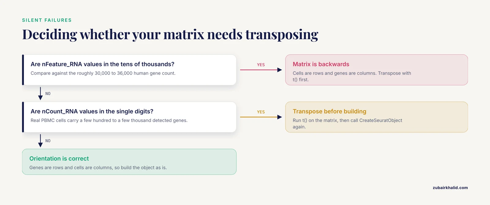
Symptom: nFeature_RNA values in the tens of thousands, nCount_RNA values in the single digits. This means your matrix was cells by rows instead of genes by rows. Fix: transpose with t() before CreateSeuratObject. This is the single most common failure when importing CSV files.

Error: "No features match this pattern"

Warning: No features match this pattern. Skipping mitochondrial percentage calculation.

Cause: gene identifiers in the matrix are Ensembl IDs, so the pattern ^MT- finds nothing. Fix: map Ensembl IDs to gene symbols with biomaRt or use the features.tsv file from CellRanger, which contains both identifiers [1]. Without symbol-level identifiers, mitochondrial QC, ribosomal QC, and most marker-based annotation will silently do nothing.

Error: duplicate row names

Error in rownames<- : duplicate 'rownames' are not allowed

Cause: the input table has the same gene symbol on multiple rows. Fix: aggregate duplicates with AggregateExpression-style logic or collapse rows by taking row sums, or use unique Ensembl IDs as row names instead of symbols.

Error: h5 file version mismatch

Error in H5Dread: Read failure. Incompatible file format.

Cause: some providers write HDF5 matrices in formats older Seurat versions cannot read. Fix: upgrade Seurat to the current CRAN release, or fall back to the three-file mtx format, which all versions handle.

Error: RAM exhaustion during loading

Error: cannot allocate vector of size ...

Cause: a dense matrix conversion exceeded available memory. Fix: avoid as.matrix() on large sparse inputs, load mtx directly with Read10X, or use h5, or process samples one at a time before merging.

How to Check That Your Object Is Correct

A built object is not automatically a correct object. Run these five checks on every new object before analysis:

1. Dimensions are plausible. dim(pbmc) should show roughly the gene count of your reference genome (around 30,000 to 36,000 for human) and the cell count reported by CellRanger or your provider. A cell count far below the sequencing report suggests a filtering step ran twice.
2. Counts per cell land in a sane range. summary(pbmc$nCount_RNA) for human PBMCs typically shows medians in the low thousands of UMIs. Cells with single-digit UMIs are empty droplets that survived min.features if you set it too low.
3. Gene symbols look like gene symbols. head(rownames(pbmc)) should show names such as MS4A1 or CD3D, not numbers or Ensembl IDs, unless you deliberately chose IDs.
4. Mitochondrial genes are present. grep("^MT-", rownames(pbmc), value = TRUE) should return the 13 human mitochondrial genes. This check matters because mitochondrial percentage is the standard first QC metric in virtually every published scRNA-seq workflow.
5. Metadata labels match design. table(pbmc$orig.ident) should show the expected number of cells per sample, matching your channel plan.

A concrete QC pass on a fresh object:

pbmc[["percent.mt"]] <- PercentageFeatureSet(pbmc, pattern = "^MT-")
VlnPlot(pbmc, features = c("nFeature_RNA", "nCount_RNA", "percent.mt"), ncol = 3)

Cells above roughly 5 to 10 percent mitochondrial reads, or with anomalous gene counts, are candidates for removal. The exact cutoffs depend on tissue and protocol, and kidney, tumor, and cultured cell datasets differ substantially [1].

Sensible Next Steps After the Object Is Built

Once the object exists and passes QC, the standard path is normalization, feature selection, dimensionality reduction, clustering, and annotation. From there, the object becomes the substrate for specialized analyses. If your experiment included immune receptor enrichment, packages such as scRepertoire attach TCR and BCR clonotype data derived from 10x Immune Profiling output directly onto the Seurat object [10]. If your data includes protein measurements from antibody oligos, weighted-nearest-neighbor integration lets Seurat combine RNA and protein modalities into a single cellular state definition [2]. If your long-term aim is deconvolution of bulk RNA-seq using single-cell references, the Seurat object is the standard intermediate from which reference profiles are extracted [11].

If you work primarily in the Bioconductor ecosystem, note that equivalent containers exist. The Voyager project, implemented in R/Bioconductor, operates on data structures that combine gene expression matrices with spatial geometries, and it maintains reproducible tutorials built on automated continuous integration [5]. Knowing both ecosystems widens the set of methods available to you, especially for spatial transcriptomics where Voyager brings geospatial statistics to single-cell data [5][4].

Common Mistakes and Limitations

• Transposed matrices. The most frequent silent failure. If nFeature_RNA per cell equals your gene count, the matrix is backwards. Transpose before construction.
• Filtering twice. Some pipelines hand you already-filtered matrices, and applying aggressive min.features on top can remove real cells. Check the CellRanger web summary for expected cell counts [1] before filtering.
• Confusing raw and filtered folders. CellRanger writes both raw_feature_bc_matrix (all barcodes, mostly empty) and filtered_feature_bc_matrix (cell-associated barcodes) [1]. Loading the raw folder without min.features gives you an object dominated by empty droplets.
• Assuming the object is analysis-ready. A freshly created Seurat object contains raw counts only. Normalization, scaling, and dimensionality reduction have not happened. Analyses run on raw counts directly will not reproduce published results.
• Treating default thresholds as tissue-universal. min.features = 200 is reasonable for PBMCs. Tissues with low RNA content, or organisms with compact genomes such as yeast, where 10x protocols were adapted with specific lysis modifications, may need different thresholds [12].
• Overwriting assay slots with normalized values. Keep raw counts in the counts layer and normalized data in data. Objects that lose raw counts cannot be re-analyzed with newer methods later.
• Memory underestimation. Published cohort-scale projects process hundreds of thousands of cells, and RCC tumor atlas work annotated hundreds of thousands of high-quality cells across dozens of samples [13]. Plan RAM accordingly and split large loads into per-sample objects before merging.
• Individual analysis decisions vary by dataset. Threshold choices, feature selection numbers, and clustering resolutions are dataset dependent. Published end-to-end analyses, including clinical studies that created Seurat objects from GEO-deposited data, adjusted these parameters to their own data rather than copying defaults blindly [3].

Frequently Asked Questions

What does a Seurat object actually contain?

It contains a raw count matrix in an assay slot, per-cell metadata, per-gene metadata, and empty slots that later fill with normalized data, variable features, dimensionality reductions, and graphs. Printing the object shows which slots are populated.

Can I create a Seurat object from a CSV file?

Yes. Read the CSV with row names set to gene identifiers, convert to a sparse dgCMatrix, confirm genes are rows and cells are columns, and pass the matrix to CreateSeuratObject. Transpose first if the orientation is wrong.

Do I need CellRanger before creating a Seurat object?

If your data is 10x Genomics FASTQ output, yes, CellRanger or an equivalent aligner and counter produces the count matrix you load [1]. If you received a matrix from a collaborator or GEO, CellRanger already ran and you can start directly.

What are min.cells and min.features doing?

min.cells removes genes detected in fewer than that many cells, and min.features removes cells expressing fewer than that many genes. Both are first-pass filters applied during object construction, and both are tunable per tissue.

How do I create a Seurat object from multiple samples?

Build one object per sample with a distinct project label, then combine them with merge() using add.cell.ids to prevent barcode collisions. The orig.ident metadata column preserves sample identity through the merge.

Is a Seurat object the same as a SingleCellExperiment object?

No, but they are equivalent containers from different ecosystems. Seurat is CRAN-based and used by the Satija Lab toolkit, while SingleCellExperiment is Bioconductor's standard and underlies packages such as Voyager [5]. Conversion functions exist in both directions.

Why does my object show fewer genes than expected?

min.cells filtering removes lowly detected genes during construction, and the default Read10X behavior with CellRanger feature files includes all features in the reference, not all of which pass filtering. A gene count of 20,000 to 25,000 after filtering is normal for a 10x human dataset.

Can Seurat handle multimodal data like CITE-seq?

Yes. Pass a named list from Read10X where each element is a feature type, and create separate assays. The weighted-nearest-neighbor framework in Seurat then integrates RNA and protein measurements into unified cell state definitions [2].

Sources

1. Single cell RNA sequencing (scRNA-seq) v1
2. Integrated analysis of multimodal single-cell data
3. Integrating single-cell and bulk RNA sequencing to predict prognosis and immunotherapy response in prostate cancer.
4. Opportunities and challenges of single-cell and spatially resolved genomics methods for neuroscience discovery
5. Voyager: exploratory single-cell genomics data analysis with geospatial statistics
6. scraps: an end-to-end pipeline for measuring alternative polyadenylation at high resolution using single-cell RNA-seq
7. Highly Multiplexed Single-Cell Full-Length cDNA Sequencing of human immune cells with 10X Genomics and R2C2
8. SEACells infers transcriptional and epigenomic cellular states from single-cell genomics data
9. Detection of PatIent-Level distances from single cell genomics and pathomics data with Optimal Transport (PILOT)
10. scRepertoire: An R-based toolkit for single-cell immune receptor analysis
11. Cell composition analysis of bulk genomics using single cell data
12. Single-Cell RNA Sequencing in Yeast Using the 10× Genomics Chromium Device.
13. Investigation of tumor-associated macrophages (TAMs) and therapeutic resistance to immune checkpoint inhibitors (ICI) through single-cell analysis of renal cell carcinoma (RCC).