How to Convert Between Genomic Data Formats in R

By Dr. Zubair Khalid, DVM, MS, PhD · 2026-11-11

By the end of this guide you will be able to move sequencing reads, variant calls, genotype matrices, genomic intervals, chromatin interactions, single-cell objects, and large count matrices between the file formats that different analysis tools expect, using R for every step. You will know which package handles which conversion, the exact commands to run, what a correct result looks like, and how to verify that nothing was lost or shifted along the way.

You need R 4.4 or newer, the BiocManager installer, and a few gigabytes of free disk space for the examples. Most of the heavy lifting comes from Bioconductor, the open-source project that supplies the majority of R's genomics infrastructure, so this guide also works as a compact Bioconductor tutorial focused on conversion work. The small examples run on a laptop. The disk-backed approaches in Steps 3, 5, and 9 exist precisely for files that exceed memory.

Install everything once, up front:

if (!requireNamespace("BiocManager", quietly = TRUE)) {
  install.packages("BiocManager")
}
BiocManager::install(c(
  "ShortRead", "VariantAnnotation", "rtracklayer", "GenomicRanges",
  "GenomicFeatures", "InteractionSet", "GWASTools", "Zellkonverter",
  "HDF5Array", "tidyCoverage"
))
install.packages(c("vcfR", "adegenet", "data.table", "Matrix"))

Why Genomic Data Comes in So Many Formats

Each tool community standardized on the file format that suited its hardware and its questions, and those choices persist long after the hardware changed. Knowing what each format stores is the first step in converting it well.

FASTQ is the text format for raw sequencing reads. Each record has four lines, an identifier, the DNA sequence, a separator, and per-base quality scores encoded as characters. ShortRead handles input, quality assessment, manipulation, and output of high-throughput sequence data in R [1].

SAM and BAM store read alignments to a reference genome. SAM is tab-delimited text, BAM is its compressed binary twin. Alignment-to-BAM conversion usually happens with samtools in the shell, and published RNA-seq protocols convert, sort, and index alignments with samtools before handing data to R for counting and statistics [2].

VCF and BCF describe genetic variants. The Variant Call Format records chromosome, position, reference and alternate alleles, per-sample genotypes, and annotations. BCF is the binary, compressed counterpart.

BED is a tab-delimited interval format, chromosome, start, end, used by genome browsers and peak callers. GFF and GTF are one-based annotation formats for genes, transcripts, and exons. BigWig and BigBed are compressed, indexed binary formats for per-base signals such as coverage and for dense interval sets.

PLINK files come in two generations, the older .ped and .map text pair and the newer binary .bed, .bim, .fam trio. Many analysis platforms expect the binary form. EigenGWAS, for example, accepts PLINK binary format that has been converted from original sequencing data [3].

Genepop is a multilocus text format from population genetics, with individuals grouped by population and alleles coded as three-digit numbers.

RDS is R's native serialization for a single object. H5AD is an HDF5 file holding an AnnData object from the Python single-cell ecosystem. HDF5, NetCDF, and SQLite are disk-backed containers, meaning the data stay on disk and R reads pieces on demand, which is how modern tools handle datasets larger than memory [2].

R for bioinformatics earned its place in conversion work because Bioconductor defines hub containers, chiefly GRanges for intervals and SummarizedExperiment for matrices with row and column metadata, that nearly every other format can be mapped into and back out of.

The Core R Packages for Format Conversion

Four step flow: a source file read into GRanges, coordinates shifted by one, then written out to the target format.

The table below is the map for everything that follows. Keep it open while you work.

From	To	Package	Key functions	Watch out for
FASTQ	subsets, QA reports	ShortRead	readFastq, writeFastq, FastqStreamer, qa	stream large files instead of loading them [1]
VCF	genotype matrix, data frame	VariantAnnotation, vcfR	readVcf, geno, read.vcfR, extract.gt	genome build and ploidy
VCF, BCF, PLINK, IMPUTE2	SQLite, then data frames	Mega2R	database loaders, gene-based test wrappers	run the Mega2 C++ step first [4]
Genepop	other software formats	genepopedit	diagnostic and transformation functions	three-digit allele coding [5]
PLINK and sequencing calls	NetCDF containers	GWASTools	NetCDF readers, GenotypeData	disk-backed, not in-memory [6]
BED, GFF, BigWig, BigBed	GRanges	rtracklayer	import, export	0-based versus 1-based coordinates
BEDPE	GInteractions	InteractionSet	GInteractions	add 1 to BED starts [7]
RDS, SingleCellExperiment	H5AD and back	Zellkonverter	writeH5AD, readH5AD	metadata type drift [8]
in-memory matrix	HDF5	HDF5Array	writeHDF5Array	memory and speed trade-offs [9]
coverage tracks	tidy frames	tidyCoverage	CoverageExperiment	needs R 4.4 and Bioconductor 3.19 [10]

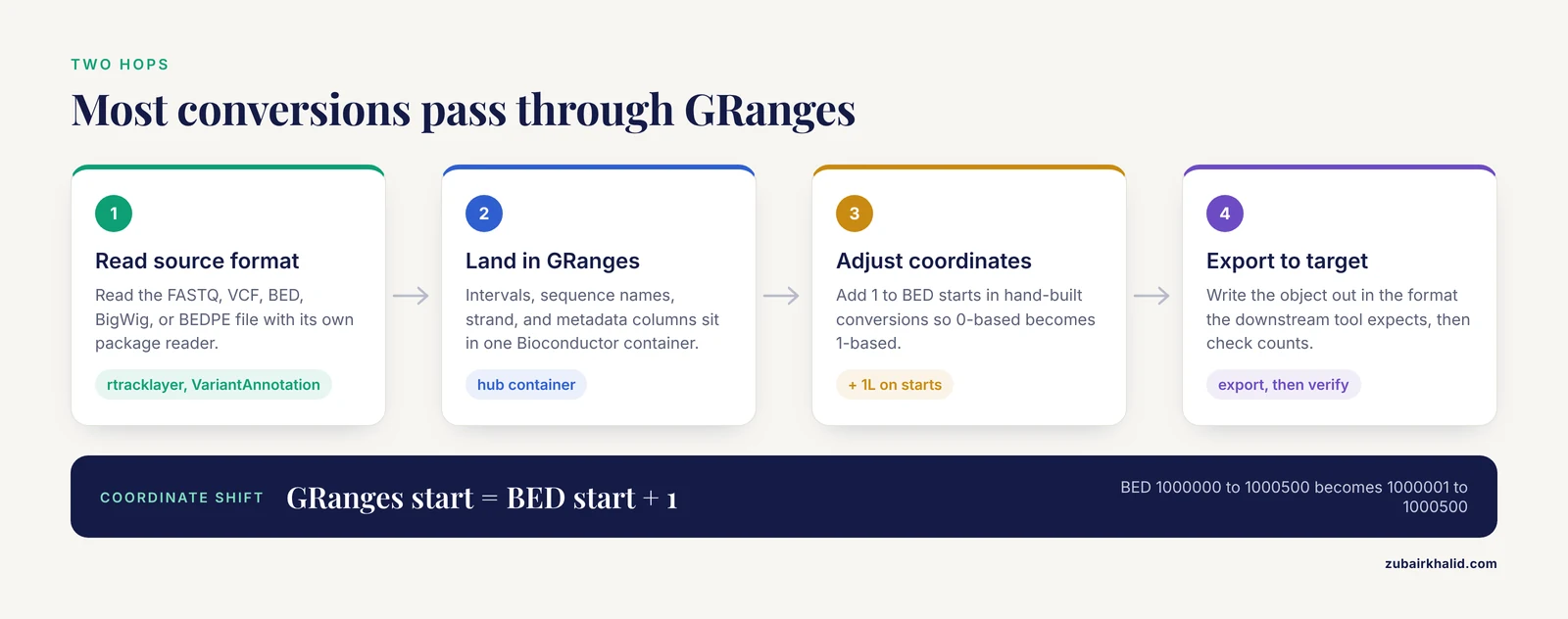
GRanges is the workhorse in this table. It is Bioconductor's standard container for genomic intervals, holding sequence names, ranges, strand, and metadata columns in one object. Most conversions in practice are two hops, source format to GRanges, then GRanges to destination format.

Convert Genomic Data Formats in R, Step by Step

The ten steps below cover the conversions that come up most often. Each one shows the command, the expected shape of the output, and the detail that trips people up.

Step 1: FASTQ reads with ShortRead

ShortRead reads gzipped FASTQ directly, assesses quality, and writes FASTQ back out [1].

library(ShortRead)

fq <- readFastq("sample_R1.fastq.gz")
fq
# class: ShortReadQ
# length: 250000 reads
# width: 150 cycles

sread(fq)[1:2]
# A DNAStringSet instance of width 150
# [11] GATCGATC...
# [4] CCTACCTA...

quality(fq)[1:2]
# A BStringSet instance of width 150
# [11] +FF,FHHH...

Write a subset back out, keeping the .gz extension so the output stays compressed:

writeFastq(fq[1:10000], "subset_R1.fastq.gz")

For files too large to hold in memory, stream in fixed-size chunks with FastqStreamer. Each call to yield returns the next block of reads:

streamer <- FastqStreamer("sample_R1.fastq.gz", n = 1000000)
repeat {
  chunk <- yield(streamer)
  if (length(chunk) == 0) break
  # process the chunk, for example count reads or trim bases
}
close(streamer)

For a quality overview before or after conversion, run the built-in assessment and write the HTML report:

qa_summary <- qa("sample_R1.fastq.gz", type = "FastqQuality")
report(qa_summary, "qa_report")

One boundary to respect here, ShortRead ends at FASTQ. Converting SAM to BAM, sorting, and indexing belong to samtools in the shell, which is how published RNA-seq protocols arrange it before R takes over for counting and statistics [2].

Step 2: VCF to genotype matrices and data frames

VariantAnnotation reads VCF into a CollapsedVCF object and exposes genotypes through the geno accessor:

library(VariantAnnotation)

vcf <- readVcf("variants.vcf.gz", genome = "GRCh38")
vcf
# class: CollapsedVCF
# dim: 12045 28
#   12045 variant rows, 28 samples

gt <- geno(vcf)$GT
head(gt[, 1:3])
#        HG00096 HG00097 HG00099
# rs6054257 "0/1"   "1/1"   "0/0"

The fixed fields become a plain data frame when you need one:

fixed_df <- as.data.frame(fixed(vcf))
head(fixed_df[, c("REF", "ALT", "QUAL")])
#   REF  ALT  QUAL
# 1   G    A   288
# 2   T    C    74

Most downstream tools want genotypes as an integer allele dosage matrix, 0, 1, or 2 copies of the alternate allele. Convert the GT strings yourself so the rule is explicit:

to_dosage <- function(x) {
  x <- gsub("|", "/", x, fixed = TRUE)
  alleles <- strsplit(x, "/", fixed = TRUE)
  vapply(alleles, function(a) sum(a == "1"), integer(1))
}
alt_dosage <- apply(gt, 2, to_dosage)
head(alt_dosage[, 1:3])
#            HG00096 HG00097 HG00099
# rs6054257        1       2       0

This function assumes biallelic diploid sites. Ploidy is a real conversion decision, not a detail. Researchers working with tetraploid genotyping-by-sequencing data wrote an R script that converts VCF records into diploidized genotype calls, and their power analysis shows why the distinction matters, 17 reads suffice to classify a simplex tetraploid heterozygote with 95 percent accuracy while allele dosage calls need 61 reads [12].

The vcfR package is a lighter alternative that many population geneticists prefer:

library(vcfR)
vcf_obj <- read.vcfR("variants.vcf.gz")
gt_mat <- extract.gt(vcf_obj)
head(gt_mat[, 1:3])

From there, adegenet converts straight into its genlight container for population-level analyses:

library(adegenet)
genlight_obj <- vcfR2genlight(vcf_obj)

To write VCF back out, use writeVcf, which preserves the header and sample columns:

writeVcf(vcf, "variants_converted.vcf.gz")

Step 3: VCF, BCF, PLINK, and IMPUTE2 through Mega2R

When the destination is one of the classic linkage or association programs, Mega2R is the bridge. The Mega2 program converts data from several genetic data formats, including PLINK, VCF, BCF, and IMPUTE2, into the specific requirements of more than 40 analysis programs, and it now uses a SQLite database as its intermediate representation. The Mega2R package loads that database directly into R as data frames and keeps biallelic genotypes in a compressed form, expanding portions only when a function needs them [4].

library(Mega2R)
# The workflow is always the same three moves:
#   1. Outside R, run the Mega2 C++ program once to build a SQLite
#      database from your PLINK, VCF, BCF, or IMPUTE2 input.
#   2. Point Mega2R at the database file.
#   3. Work with the tables as data frames, or call the built-in
#      wrappers that loop over genes to run pedgene and SKAT
#      gene-based association tests directly from the database [4].

The exact call for opening a database is documented in the Mega2R vignette and changes slightly between versions, so read the vignette shipped with your installed copy rather than copying an old script.

Step 4: Genepop population files with genepopedit

A Genepop file has a title line, then blocks per population, then individual lines with three-digit allele codes per locus:

GPDipDemo
Pop
Ind_001  010203 010204 030404
Pop
Ind_002  010203 020204 030404

genepopedit was built for exactly this format. Its functionality divides into diagnostic, manipulation, sampling, simulation, and transformation tools, it extracts metadata from large files without opening them in a text editor, and it converts directly to a variety of software-specific formats. The authors report it stays stable for datasets in excess of 200,000 SNPs [5].

library(genepopedit)
# Typical conversion flow, one function per job:
#   1. Diagnostics: summarize loci, samples, and populations.
#   2. Manipulation: drop unwanted loci or individuals.
#   3. Transformation: write the cleaned file into the input
#      format of the downstream program.
# Use ?genepopedit to list the functions available in your
# installed version, then chain them in a single script [5].

The value here is repeatability. The same script rerun next month produces the same file, which manual editing in a text editor never guarantees.

Step 5: GWAS genotypes into disk-backed containers with GWASTools

Genome-wide association datasets routinely outgrow RAM. GWASTools stores genotypes in NetCDF format to accommodate extremely large datasets that cannot fit within R's memory limits, and its documentation includes instructions for converting data from multiple formats, including variants called from sequencing [6].

library(GWASTools)
# GWASTools keeps genotype and intensity data in NetCDF files on disk,
# then exposes them through reader classes that behave like ordinary
# in-memory objects. The package documentation walks through converting
# PLINK text, plain text matrices, and sequencing-derived calls into
# its NetCDF containers [6].

If the destination is a GWAS scanner rather than an R container, prepare PLINK binary format. EigenGWAS accepts PLINK binary directly, and its documentation notes that this format is easily converted from original sequencing data [3].

Step 6: BED, GFF, and BigWig tracks with rtracklayer

rtracklayer imports BED, GFF, BEDGraph, WIG, BigWig, and BigBed files into GRanges and exports GRanges back into those formats:

library(rtracklayer)

peaks <- import("chip_peaks.bed")
peaks
# GRanges object with 3 ranges and 2 metadata columns:
#     seqnames            ranges strand |     name     score
#        <Rle>         <IRanges>  <Rle> | <factor> <numeric>
#   [11]     chr1   1000001-1000250      + |   peak_1        42
#   [4]     chr1 25300001-25300400      - |   peak_2        87
#   [5]     chr2     500001-500150      + |   peak_3        55

export(peaks, "chip_peaks.gff3")

For a continuous signal track, restrict the import to the regions you actually need, which keeps memory use small:

signal <- import("chip_signal.bw", which = peaks[11])
head(signal)

For gene annotation in GTF form, GenomicFeatures builds a transcript database directly from the file:

library(GenomicFeatures)
txdb <- makeTxDbFromGFF("genes.gtf")

Coverage tracks deserve their own container. tidyCoverage defines CoverageExperiment and AggregatedCoverage classes, both extending SummarizedExperiment, to extract and manipulate genome-wide track data across thousands of loci at once, and it requires R 4.4 or newer with Bioconductor 3.19 or newer [10].

Step 7: Chromatin interactions with InteractionSet and GenomicInteractions

Hi-C and ChIA-PET experiments produce interactions between pairs of loci, usually exchanged as BEDPE files. InteractionSet provides the Bioconductor classes that represent genomic interactions and their associated experimental data, built on existing infrastructure and reused by higher-level packages, which improves interoperability across the ecosystem [7].

Convert a BEDPE file by hand so the coordinate shift is visible:

library(InteractionSet)
library(data.table)

bedpe <- fread("loops.bedpe")
head(bedpe)
#     chr1    start1      end1  chr2    start2      end2
#   <char>     <int>     <int> <char>     <int>     <int>
# 1:   chr1   1000000   1000500   chr1 12000000 12000500
# 2:   chr1  25300000  25300500   chr2    50000    500500

gi <- GInteractions(
  GRanges(bedpe$chr1, IRanges(bedpe$start1 + 1L, bedpe$end1)),
  GRanges(bedpe$chr2, IRanges(bedpe$start2 + 1L, bedpe$end2))
)
gi
# GInteractions object with 2 interactions and 0 metadata columns:
#       seqnames1         ranges1   seqnames2         ranges2
#           <Rle>       <IRanges>       <Rle>       <IRanges>
#   [11]      chr1 1000001-1000500       chr1 12000001-12000500
#   [4]      chr1 25300001-25300500       chr2   500001-500500

The + 1L on each start column is not decoration. BED coordinates are 0-based and half-open, GRanges coordinates are 1-based and inclusive, so skipping the shift moves every anchor one base upstream. GenomicInteractions then handles the analysis side, providing annotation, summarization, and visualization methods for chromosome conformation capture data, demonstrated on Hi-C and ChIA-PET datasets [11].

Step 8: Single-cell objects between RDS and H5AD

Three question decision path for choosing between RDS and H5AD when sharing single-cell data, ending in a type recheck.

Single-cell data crosses between the R and Python ecosystems constantly, and Zellkonverter is the standard Bioconductor bridge:

library(Zellkonverter)
library(SingleCellExperiment)

sce <- readRDS("pbmc_tumor.rds")
writeH5AD(sce, "pbmc_tumor.h5ad")

sce_back <- readH5AD("pbmc_tumor.h5ad")
identical(dim(sce), dim(sce_back))
# [11] TRUE

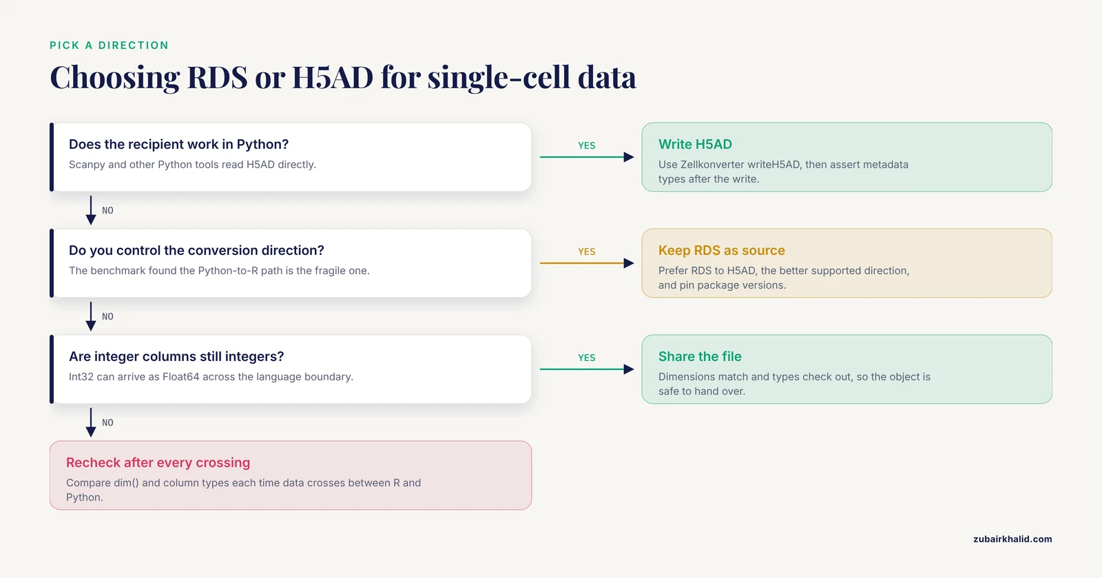
Conversion reliability is not uniform, and a systematic benchmark of five conversion tools across 68 datasets ranging from 1,438 to 1,665,937 cells found a substantial gap in H5AD-to-RDS conversion, meaning the Python-to-R direction is the fragile one. Cross-language boundaries introduce implicit type changes, such as Int32 becoming Float64, that can break downstream code expecting integers. The same benchmark found existing tools failing on datasets well below 74,000 cells in some cases, and reported that the Rust-based CrossCell toolkit achieved 100 percent success across 55 standard datasets with 2.5 to 4.9 times the speed and 37 to 61 percent memory savings, scaling to 13 CELLxGENE datasets up to 1.67 million cells [8].

The practical translation, pin your package versions, prefer RDS to H5AD when you control the direction, and verify metadata types after every crossing.

Step 9: Large matrices to HDF5

Count matrices from single-cell and bulk experiments are often sparse, meaning most entries are zero and only nonzero values are stored. When even the sparse form is too big, write the matrix to HDF5 and let R read it lazily:

library(HDF5Array)

counts <- matrix(rpois(20000, 5), nrow = 2000)
dimnames(counts) <- list(paste0("gene_", 1:2000), paste0("cell_", 1:10))

counts_h5 <- writeHDF5Array(counts, "counts.h5", name = "counts")
counts_h5
# <2000 x 10> HDF5Array object of type "integer"

The returned HDF5Array behaves like a matrix but reads blocks from disk on demand. For package developers, beachmat defines a C++ interface that reads dense, sparse, and file-backed matrices through one API, and its performance evaluation on real and simulated scRNA-seq data defined a clear memory and speed trade-off to guide the choice of representation [9]. The consequence for everyday work is pleasant, code written against beachmat-compatible interfaces does not require you to physically convert a matrix before analyzing it.

Step 10: Proteomics conversions with SWATH2stats and mzML

Format conversion is not exclusive to nucleotides. In proteomics, SWATH2stats processes OpenSWATH output into a format directly readable by downstream statistical tools such as MSstats, mapDIA, and aLFQ, adding annotation, FDR estimation, and filtering before submission [13].

library(SWATH2stats)
# SWATH2stats reads OpenSWATH output tables, annotates and filters them,
# and writes files that MSstats, mapDIA, and aLFQ ingest directly [13].

At the raw end of the pipeline, the MASSyPupX collection converts Thermo raw files downloaded from ProteomeXchange into the HUPO community format mzML, then hands the results to Bash, Python, and R scripts for post-processing and visualization [14]. The lesson transfers to genomics, conversion tools often live one step upstream of R, and a good workflow knows where the boundary sits.

How to Check That a Conversion Worked

A conversion that runs without errors can still be wrong. Build these checks into every script.

Compare record counts. The number of variants, reads, intervals, or cells should match across the boundary, or differ for a reason you can state.

dim(vcf)
dim(sce_back)
identical(dim(sce), dim(sce_back))
# [11] TRUE

Spot-check the first and last records against the original file opened in a pager or a spreadsheet. Look at identifiers, not just row counts.

Round-trip when the format allows it. Write, read back, and compare:

export(peaks, "roundtrip.bed")
peaks_back <- import("roundtrip.bed")
all.equal(as.data.frame(peaks), as.data.frame(peaks_back))
# [11] TRUE

Verify one known landmark. Take a variant or gene with a published position and confirm it lands at the same coordinate after conversion. This catches genome build and coordinate-system errors that counts never will.

Assert metadata types after cross-language conversion, because integer columns can arrive as floating point [8].

Record the environment with sessionInfo() and save it next to the output file. A conversion is only reproducible if you know which package versions produced it.

Tips for Reliable Conversions

These are the habits that separate a one-off hack from a workflow you can trust.

Treat raw files as read-only. Write every converted file into a derived directory, and do the conversion in a script. genepopedit exists largely because repeatable, code-based manipulation of genomic data beats manual editing, and the principle applies to every format in this guide [5].

Stream or use disk-backed containers for anything large. FastqStreamer for reads, SQLite in Mega2R [4], NetCDF in GWASTools [6], HDF5 through HDF5Array and beachmat. Loading a 40 GB file into memory to change its format is the most expensive way to do a simple job.

Pin the genome build and the sequence naming style. hg19 and GRCh37 describe the same reference with different labels, and mismatched naming silently produces empty overlaps. GenomeInfoDb fixes styles on GRanges objects:

library(GenomeInfoDb)
seqlevelsStyle(peaks) <- "UCSC"

Convert through hub containers rather than format to format. Source to GRanges, GRanges to destination, halves the number of direct conversions you need to know. Newer containers follow the same pattern, QTLExperiment stores QTL summary statistics and metadata in a Bioconductor-consistent object so multi-state QTL analyses interoperate [15].

Prefer the tidy grammar when pipelines get long. The tidyomics ecosystem bridges Bioconductor objects to tidy R manipulation, demonstrated on 7.5 million peripheral blood mononuclear cells from the Human Cell Atlas spanning six data frameworks and ten analysis tools [16].

Check ploidy and phase before converting genotypes to dosages. A diploid dosage function applied to polyploid data produces confident nonsense [12].

For single-cell exchange, fix the direction deliberately. The R-to-Python path is the better supported one, and type checks after conversion are cheap insurance [8].

Read the receiving tool's input specification before writing the file. Most conversion failures are specification mismatches, a missing header line, an unsupported allele code, an unexpected compression, not bugs in your R code.

Common Mistakes and Limitations

Confusing the two BEDs. PLINK's binary genotype file is called .bed, and UCSC's Browser Extensible Data is also called .bed. They share nothing but the extension. Opening a PLINK .bed in a genome browser or with rtracklayer produces garbage or an error, and the mistake is common enough that every conversion script should record which BED it means.

Off-by-one coordinate shifts. BED is 0-based and half-open, so a BED interval written as 1000000 to 1000500 covers bases 1000001 through 1000500 in 1-based systems. GFF, GTF, and VCF are 1-based. rtracklayer handles the shift on import and export, but hand-built conversions, like the BEDPE example in Step 7, must add 1 to starts explicitly. A one-base error can move an interval off an exon boundary or a restriction site, and nothing downstream will complain.

Genome build mismatches. Converting coordinates from one build to another is a different job from converting formats, and confusing the two is a classic error. A file labeled hg19 but containing GRCh38 coordinates will import cleanly and analyze wrongly. Always verify a known landmark position after conversion.

Silent type changes across languages. When single-cell objects cross between R and Python, integer columns can arrive as floating point because of implicit type changes at the language boundary [8]. Code that expects integer cell barcodes or integer counts can misbehave without an error message. Assert types after conversion.

Direction asymmetry in single-cell conversion. The benchmark evidence points one way, RDS to H5AD is the reliable direction, H5AD to RDS is where tools struggle [8]. Plan your sharing direction around this.

Loading giant files into memory. Reading a whole FASTQ, VCF, or count matrix to convert it wastes hours and crashes sessions. Streaming and disk-backed containers exist for this exact reason.

Assuming conversion validates data. Conversion moves bytes between formats. It does not fix low-quality genotype calls, missing strand information, duplicate identifiers, or the wrong genome build. Those problems travel faithfully into the new format.

Dropping records at format boundaries. Moving VCF data into genotype-oriented tools can drop multiallelic sites, indels, or sites failing implicit filters. Compare record counts before and after, and account for every difference.

A limitation worth stating once. Format conversion is plumbing, and correct plumbing does not make an analysis correct. Biological conclusions need domain review, and any result bearing on health decisions needs evaluation by a qualified professional.

Frequently Asked Questions

What does it mean to convert genomic data formats in R?

It means reading a file such as a VCF, FASTQ, BED, or PLINK file into R, transforming it into another structure or format, and writing it out so a downstream tool can read it, using R packages instead of manual editing.

Which R package converts a VCF file to a genotype matrix?

VariantAnnotation reads VCF files and exposes genotypes through the geno accessor, and vcfR with its extract.gt function is a lighter alternative that pairs well with adegenet for population genetics work.

How do I convert a Seurat or SingleCellExperiment object to H5AD in R?

Use Zellkonverter, calling writeH5AD on your object to produce an H5AD file that Python tools such as Scanpy read directly, then verify dimensions and metadata types after the write.

Can R read PLINK files directly?

Yes, through routes such as Mega2R, which converts PLINK, VCF, BCF, and IMPUTE2 input into a SQLite database and loads it into R as data frames, and GWASTools, which documents conversion into its NetCDF containers.

How do I avoid off-by-one errors when converting BED files?

Remember that BED coordinates are 0-based and half-open while GRanges, GFF, and VCF are 1-based, add 1 to BED starts in hand-built conversions, and prefer rtracklayer import and export, which handle the shift for you.

What should I do if my FASTQ file is too large for memory?

Stream it in chunks with ShortRead's FastqStreamer, processing and writing each block with yield before the next one, so memory use stays flat regardless of file size.

Should I share single-cell data as RDS or H5AD?

Match your recipient's ecosystem, RDS for R users and H5AD for Python users, and favor the RDS to H5AD direction when you control it, because the reverse path is the one conversion tools handle least reliably.

Do I need Bioconductor to convert genomic data formats in R?

Most conversion infrastructure lives in Bioconductor, so install BiocManager and the packages listed in this guide, while a few helpers such as vcfR and data.table come from CRAN.