How to Convert Counts to TPM in R: A Practical Guide
By Dr. Zubair Khalid, DVM, MS, PhD ·

By the end of this guide you will be able to take an RNA-seq count matrix and produce a TPM (transcripts per million) matrix in R that is correctly length normalized, sums to one million per sample, and is ready for visualization, cross-sample comparison, or reporting. You will also know when TPM is the wrong scale to use and why raw counts must stay in your pipeline for differential expression analysis.
You need R 4.2 or newer, the Bioconductor packages tximport and optionally edgeR, and one of two inputs: a set of transcript quantification files from Salmon, kallisto, or RSEM, or a gene-level count matrix with a matching table of gene lengths. Modern RNA-seq workflows in R routinely move between count matrices and normalized expression matrices, and published protocols treat conversion to TPM as a standard step after read counting [1]. The key point to understand before writing any code is that TPM requires gene lengths, so a count matrix on its own is never enough.
What TPM Actually Measures
TPM stands for transcripts per million. It answers a specific question: if I sequenced one million transcripts in this sample, how many of them would come from this gene? The answer accounts for two technical facts about RNA-seq.
First, samples are sequenced to different depths. A gene in a sample sequenced at 20 million reads will show roughly twice the count of the same gene sequenced at 10 million reads, even if the underlying expression is identical. Dividing by a per-million scale factor removes this library size difference.
Second, longer genes collect more reads. A 6 kb transcript fragments into roughly three times as many fragments as a 2 kb transcript at the same molar abundance. Dividing each gene's count by its effective length removes this bias. The effective length is the transcript length minus the average fragment length plus one, which corrects for the fact that fragments shorter than the transcript cannot start at every position. Quantification tools like Salmon and RSEM compute effective lengths internally and report them in their output files.
The TPM formula is applied in two passes per sample:
1. rate_i = counts_i / effective_length_i          (for every gene i)
2. TPM_i  = rate_i / sum(rate_j) * 1,000,000       (sum over all genes j)
Because the denominators in step 2 are summed within each sample, TPM values always add up to one million per sample. This property is the fastest sanity check that your conversion worked, and it is also the reason TPM is called a relative measure. It describes the composition of the transcriptome in each sample, which matters when you interpret cross-sample comparisons.
Raw count data behave very differently from TPM. Counts are discrete, highly skewed, and in settings such as miRNA-seq they can span from zero to millions within one dataset, which is why statistical models built for counts, such as the negative binomial, exist in the first place [3]. TPM is a continuous, normalized scale, and confusing the two is the single most common error in this workflow.
TPM, RPKM, and CPM: A Comparison You Can Code Against
Before writing code, it helps to see how the three common normalizations differ. All three correct for library size, but only TPM and RPKM correct for gene length, and only TPM normalizes length first and depth second, which makes TPM values comparable between samples in a way RPKM values are not.
| Measure | Formula (per gene, per sample) | Corrects for depth | Corrects for length | Sums to a constant per sample | Typical use |
|---|---|---|---|---|---|
| TPM | rate / sum(rate) × 10^6, rate = counts / effective length | Yes | Yes | Yes (10^6) | Cross-sample visualization, reporting abundance |
| RPKM | counts / (length in kb × mapped reads in millions) | Yes | Yes | No | Legacy single-sample length normalization |
| CPM | counts / library size × 10^6 | Yes | No | Yes (10^6) | Filtering and plotting in edgeR workflows |
The ordering matters. In RPKM you divide each gene's count by length and by total reads, so the per-sample totals of RPKM values differ across samples. In TPM you divide by length first and then rescale so the sample total is fixed at one million, which is why two samples with identical transcript composition produce identical TPM for every gene regardless of depth. If you plan to compare expression profiles across many samples, such as building a large expression atlas, TPM is the scale that keeps those profiles comparable [4].
One more distinction matters in practice. Standard library-size corrections for differential expression, including the methods implemented in packages such as TCC and the clustering-based pipelines built on them, operate on counts rather than TPM [5]. Recent work has even shown that residual library size effects can persist in normalized counts and proposed gene-specific correction terms to address it [6]. None of these methods consume TPM. Keep both scales in your workflow and use each for its intended purpose.
What You Need Installed
Open R and install the packages once:
if (!requireNamespace("BiocManager", quietly = TRUE)) {
  install.packages("BiocManager")
}
BiocManager::install(c("tximport", "edgeR"))
tximport is the Bioconductor workhorse for importing transcript quantification output and summarizing it to the gene level [7]. It handles Salmon, kallisto, RSEM, Sailfish, and several other quantifiers from a single interface, which is why most Bioconductor tutorials start differential expression workflows with a tximport step [4]. edgeR is not required for the TPM conversion itself, but it is the natural next step for differential expression on the raw counts you keep alongside TPM [8].
You also need one of these inputs:
- A
quant.sffile (or kallistoabundance.h5, or RSEM output) per sample, produced by transcript-level quantification, plus atx2genedata frame mapping transcript IDs to gene IDs. - A gene-level count matrix from featureCounts, HTSeq, or similar, plus a matching vector or column of gene lengths in the same gene ID namespace.
Everything below assumes your sample sheet is a data frame called samples with a column sample_id and, for the Salmon route, that the quant.sf files live in per-sample directories.
Step-by-Step: Convert Counts to TPM in R
Step 1. Load your sample table and check the files exist
library(tximport)

samples <- read.csv("samples.csv")
head(samples)

files <- file.path("salmon", samples$sample_id, "quant.sf")
names(files) <- samples$sample_id
all(file.exists(files))
The last line should print TRUE. If it prints FALSE, the most common causes are a mismatch between the sample_id column and the actual directory names, or missing file extensions. Fix this now, because tximport stops immediately when a listed file is absent, and an unclear file path at this stage is the most frequent reason a tximport call fails on the first attempt.
Step 2. Build the tx2gene mapping
tximport needs a two-column data frame connecting transcript identifiers to gene identifiers. For Ensembl annotations you can build it from a GTF file with the rtracklayer package or download the tx2gene table directly from resources such as the Ensembl FTP site or annotation packages like TxDb objects on Bioconductor. A minimal working version looks like this:
tx2gene <- read.csv("tx2gene.csv")
head(tx2gene)
#   tx          gene_id
# 1 ENST00000456328 ENSG00000223972
# 2 ENST00000450305 ENSG00000227232
The transcript IDs in tx2gene must match the IDs in your quantification files exactly. Version suffixes are the classic trap here. Salmon output often contains ENST00000456328.2 while a GTF-derived mapping contains ENST00000456328. Handle this either by stripping versions with a regular expression on both sides or by telling tximport to ignore versions, described in Step 3.
Step 3. Import with countsFromAbundance set to lengthScaledTPM
txi <- tximport(
  files,
  type        = "salmon",
  tx2gene     = tx2gene,
  countsFromAbundance = "lengthScaledTPM",
  ignoreTxVersion = TRUE
)

names(txi)
# "abundance" "counts"    "length"    "countsFromAbundance"
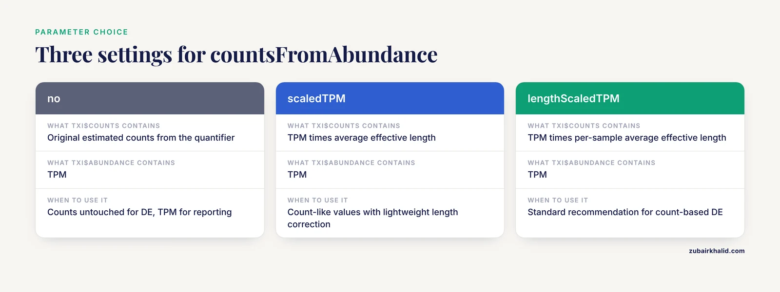
The countsFromAbundance parameter is the decision that determines whether you need any manual TPM code at all. It takes three values, explained in the table later in this section. With "lengthScaledTPM", tximport computes TPM from the abundance estimates, then multiplies TPM by the average sample effective length to produce count-like values that retain the length correction while remaining on a count scale suitable for downstream count models. The abundance element of the returned list holds TPM directly.
If you are working with pytximport in a Python pipeline, the same logic applies, because pytximport is a Python implementation of the tximport R package with the same import modes, gene-level summarization, and optional transcript-to-gene mapping generation [7]. Teams that standardize on Snakemake workflows often pick one implementation and keep both languages consistent.
For transcript-level TPM without gene summarization, set txOut = TRUE instead of supplying tx2gene:
txi_tx <- tximport(files, type = "salmon", txOut = TRUE,
                   ignoreTxVersion = TRUE)
head(txi_tx$abundance)
This returns a matrix with one row per transcript and TPM in abundance. Transcript-level output is useful for differential transcript usage and isoform-level questions, and large expression resources increasingly distribute both gene-level and transcript-level abundance matrices for exactly this reason [4].
Step 4. Extract and inspect the TPM matrix
tpm <- txi$abundance
tpm[1:5, 1:3]

colSums(tpm)
# sample_1   sample_2   sample_3
# 1000000    1000000    1000000
The column sums should equal one million, possibly with tiny floating point deviations. If a column sums to something far from one million, the import step did something you did not intend, and you should stop and inspect rather than proceed.
Step 5. The manual path: convert a gene-level count matrix to TPM
Many projects start from a count matrix rather than quantification files, for example a featureCounts output or a published count matrix downloaded from GEO. Converting counts to TPM in R in that case requires three objects: the count matrix, a vector of gene lengths in the same gene ID namespace, and the code below.
# counts: genes x samples integer matrix
# gene_lengths: named numeric vector of lengths, same row order

stopifnot(identical(rownames(counts), names(gene_lengths)))

rate <- counts / gene_lengths
tpm  <- sweep(rate, 2, colSums(rate), "/") * 1e6
The sweep call divides every column of the rate matrix by that sample's total rate, then multiplies by one million. This is the two-pass formula from the opening section, expressed in two lines of base R. Note that featureCounts reports the annotated transcript length rather than a bias-corrected effective length, so the manual route is an approximation. Quantifiers like Salmon estimate effective lengths per sample and per transcript, and one reason published resources derive TPM from quantification tools rather than from count matrices is that bias-corrected abundance estimates give more accurate differential expression results [4].
Step 6. A worked numeric example
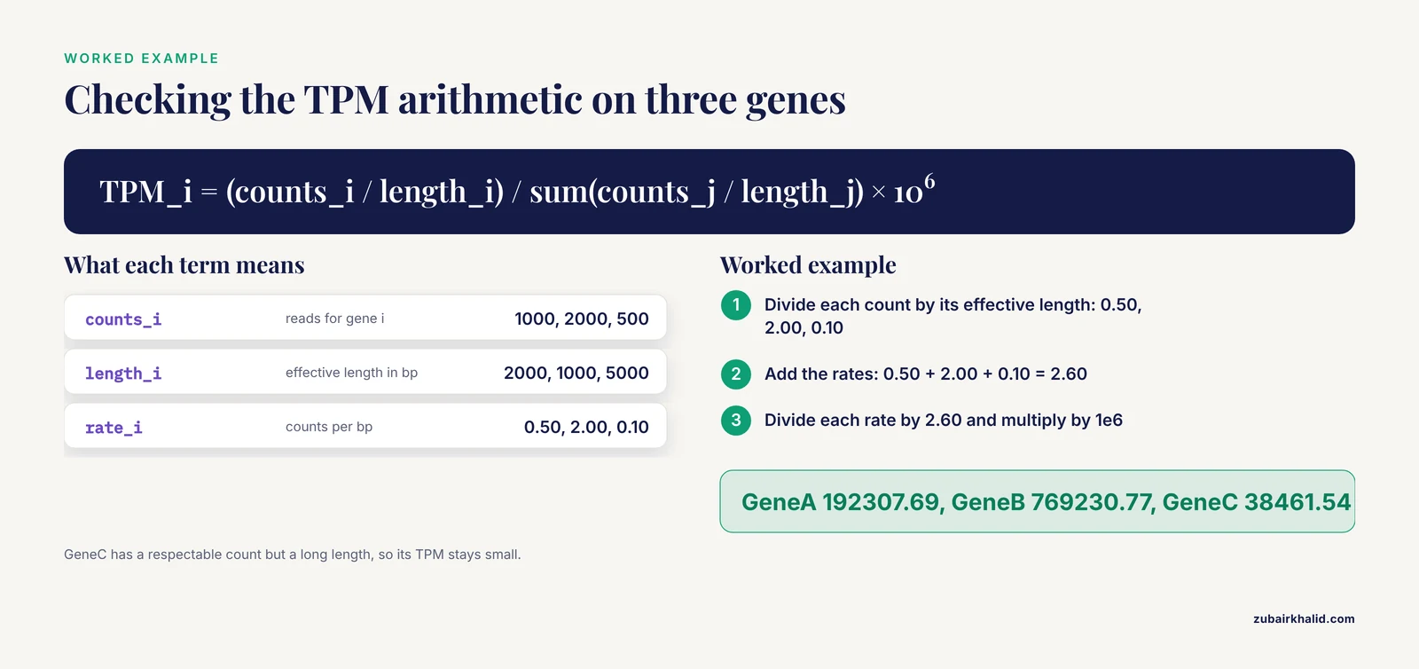
Nothing builds confidence like checking the arithmetic by hand. Take a three-gene sample sequenced at some depth and suppose the counts and effective lengths are as follows:
| Gene | Counts | Effective length (bp) | Rate (counts per bp) |
|---|---|---|---|
| GeneA | 1000 | 2000 | 0.50 |
| GeneB | 2000 | 1000 | 2.00 |
| GeneC | 500 | 5000 | 0.10 |
The rate sum is 0.50 + 2.00 + 0.10 = 2.60. Each TPM value is the gene's rate divided by 2.60, times one million:
rate <- c(1000/2000, 2000/1000, 500/5000)
tpm  <- rate / sum(rate) * 1e6
# 192307.69 769230.77  38461.54
sum(tpm)
# 1000000
GeneB is 1 kb long and pulled 2000 reads, so it dominates the sample's TPM. GeneC is 5 kb long and pulled only 500 reads, so its TPM is small despite a respectable count. If you had normalized by library size alone, GeneC would look three times closer to GeneA than it really is, because its length would never be accounted for. Run this snippet in R and confirm the output matches the values shown, and you have verified your understanding of the formula before touching real data.
Step 7. Keep the raw counts and export both
Save the raw counts before any transformation, because differential expression analysis on RNA-seq data expects count input, and this remains true whether you use edgeR, DESeq2, or a method built on top of them [9][8].
raw_counts <- txi$counts   # or your original count matrix

write.csv(raw_counts, "raw_counts.csv")
write.csv(tpm,        "tpm.csv")
saveRDS(txi,          "txi.rds")
The countsFromAbundance parameter, summarized
| Value | What txi$counts contains | What txi$abundance contains | When to use it |
|---|---|---|---|
"no" | Original estimated counts from the quantifier | TPM | You want counts untouched for DE and TPM for reporting |
"scaledTPM" | TPM × average effective length, new counts sum to original library size | TPM | Count-like values for DE with lightweight length correction |
"lengthScaledTPM" | TPM × per-sample average effective length (length-scaled counts) | TPM | Standard recommendation for count-based DE after quantification [7] |
For differential expression with DESeq2 or edgeR, "lengthScaledTPM" or "no" are the usual choices, and the DESeq2 documentation discusses lengthScaledTPM as a sensible default when transcript lengths vary across conditions. For pure TPM output, all three settings produce the same abundance matrix.
Common Errors and How to Fix Them
Error: tx2gene must be a two column data frame when running tximport with gene-level summarization. The object you passed is either a matrix, a single vector, or has more or fewer than two columns. Rebuild it with exactly two columns, transcript first, gene second, and confirm with str(tx2gene).
Transcript IDs not matching between files and tx2gene. The symptom is either an error or a silent loss of most transcripts during summarization. Check overlap directly:
quant_ids <- head(read.delim(files[10])$Name, 1000)
mean(quant_ids %in% tx2gene$tx)
If the proportion is low, inspect a few IDs from each side. Version suffixes are the usual culprit, and ignoreTxVersion = TRUE in tximport resolves the mismatch in one argument. If the mismatch is a species or genome build difference, no flag will save you and you need a consistent annotation.
Error in file(path): cannot open the connection during import. A file path is wrong. The all(file.exists(files)) check from Step 1 exists precisely to catch this before the error does, and reading the error path carefully almost always reveals a missing sample directory or an extension mismatch.
Columns of the TPM matrix do not sum to one million. The most likely cause is a manual conversion where the length vector was subset or reordered incorrectly, so some genes received the wrong lengths. Verify row alignment with identical(rownames(counts), names(gene_lengths)). A second possible cause is applying the formula to a matrix that had already been normalized once, which breaks the rate-based logic entirely.
NAs appearing after conversion. Dividing by a length of zero produces Inf or NaN. Check any(gene_lengths == 0) and decide whether to drop those features or assign them a minimum length, documenting whichever choice you make.
object 'counts' not found or unexpected coercion warnings. Count matrices read from CSV arrive as data frames, and arithmetic on data frames can silently misbehave. Coerce explicitly with as.matrix(read.csv("counts.csv", row.names = 1)) and confirm the matrix is numeric with storage.mode(counts).
Common Mistakes and Limitations
The mistakes below account for most review comments on manuscripts and most broken pipelines involving TPM.
Using TPM for differential expression. Differential expression tools model raw counts. edgeR has modeled read counts with the negative binomial distribution for over a decade and its inference framework, including the quasi-likelihood pipeline refined in version 4, is designed for count input [8]. A benchmark of eight differential analysis methods in R and Bioconductor packages, including edgeR, DESeq2, and others, evaluated all of them on count data and found no significant differences in false discovery rate control, power, or stability across methods, with DESeq2 and EBSeq leading at larger sample sizes [9]. Feeding TPM into these tools discards the count information the statistical models require and generally inflates false positives. TPM is for reporting and comparison, counts are for testing.
Confusing CPM with TPM. Dividing counts by library size and multiplying by one million produces CPM, not TPM. CPM does not correct for gene length. The two numbers can differ by orders of magnitude for short versus long genes, and a pipeline that labels CPM as TPM will produce length-biased results that look plausible on a heatmap and are wrong in every gene-level comparison.
Mixing length units across rows. Within the TPM formula, a consistent length unit cancels out, so bp and kb both work if used everywhere. The formula breaks when half the genes use one unit and half use another. One quick check is that a gene's TPM should not change when you multiply all lengths by 1000 together with the rates, and it will change if the units were inconsistent.
Summing transcript TPM to get gene TPM. Summing transcript-level TPM across the transcripts of a gene seems natural and is subtly wrong when transcripts are multi-mapped or when you want a count-consistent summary. tximport performs this summarization with the appropriate accounting, which is a core reason the Bioconductor ecosystem standardized on it [7].
Forgetting that TPM is compositional. If one highly expressed gene increases its share of the transcriptome, every other gene's TPM can decrease even with no change in its absolute expression, because TPM values must sum to one million. Compositional awareness is not pedantic. Modern frameworks built on compositional transformations of RNA-seq counts exist specifically because composition and absolute expression are different things [2]. If your biological question is about absolute RNA quantity per cell, TPM alone cannot answer it, and you should consider spike-ins or methods that model transcriptome composition explicitly.
Expecting TPM to remove every library size artifact. Large-scale reanalyses have shown that residual associations with library size can persist in expression values even after standard correction, motivating newer gene-specific correction approaches [6]. TPM handles the dominant depth and length effects, not every technical confounder, and batch effects require their own handling regardless of your normalization.
Losing raw counts along the way. Some pipelines overwrite the count matrix with TPM in the same object and then cannot run differential expression later. Write both matrices to disk, as in Step 7. This is also a reproducibility issue, because reagents and datasets aside, a paper whose TPM values cannot be traced back to counts cannot be reanalyzed.
Treating all count distributions identically. Small RNA and miRNA-seq data are dominated by a few highly expressed features and fit heavy-tailed distributions better than the standard Poisson or negative binomial assumptions [3]. If your data are miRNA-seq, be extra cautious about which features survive filtering and how a few extreme values dominate the per-million scaling.
Where TPM Fits in a Larger RNA-Seq Workflow
It helps to see the conversion in context. A complete bulk RNA-seq pipeline moves from FASTQ files through quality control, trimming, alignment, and read counting, and then branches. One branch produces count-scale matrices for differential expression, and the other produces normalized abundance matrices such as TPM for visualization, atlas building, and reporting [1]. The TPM conversion step sits at that branch point.
Several tools package this branching for you. SeqExpressionAnalyser runs the whole path from FASTQ files through quality control, filtering, alignment, counting, and differential analysis inside one Shiny-based R application [10]. RNA-SeqEZPZ offers a point-and-click pipeline from counting through differential expression and pathway analysis with an R Shiny visualization layer [11]. These tools are useful when you want the full pipeline handled, but if you are here to understand the conversion itself, doing it explicitly with tximport and the code above teaches you the details that black-box pipelines hide.
Public expression databases illustrate how the two scales coexist at scale. The Soybean Expression Atlas v2 distributes transcript-level and gene-level abundance matrices for thousands of RNA-seq samples and provides bias-corrected counts alongside TPM-like abundance estimates, with the pipeline wrapped as a reproducible R package [4]. The pattern is deliberate. Abundance for exploration, counts for statistics, both derived from the same quantification files.
A related consideration appears when bulk RNA-seq data are used to estimate cell type composition. Cell-type deconvolution methods applied to bulk RNA-seq estimate cell proportions from expression profiles, and one study found that estimates primarily reflected the mRNA content contributed by each cell type rather than true cell counts, improving agreement with matched single-cell data from a correlation of 0.62 to 0.83 after mRNA content correction [12]. Because TPM reflects relative mRNA contribution per transcriptome, abundance-scale thinking like this is exactly what TPM encodes, and it is worth remembering when you interpret deconvolution or cross-sample TPM comparisons in heterogeneous tissues.
Sensible Next Steps
With raw counts and TPM in hand, the natural next steps are the following.
- Differential expression on the counts. Load the raw counts into edgeR, filter low-count genes, apply TMM normalization, and fit a quasi-likelihood model. edgeR's expanded version 4 adds improved support for small counts and larger datasets, differential transcript expression, and pathway-level analysis, making it a strong default for count-based testing [8]. If you are comparing method choices, the published benchmark found DESeq2 and EBSeq among the strongest performers as sample sizes grow to 6 or 12 per group [9].
- Visualization on TPM. Heatmaps, sample clustering, and per-gene boxplots belong on TPM or log2(TPM + 1), where cross-sample comparability matters.
- Advanced library size handling when needed. If your dataset shows persistent library size association in diagnostics, gene-specific exponent-corrected normalization is a recently proposed alternative to uniform scale factors [6].
- Broader expression analysis. For clustering-based identification and classification of differentially expressed genes beyond standard testing, the MBCdeg3 method provides an R function operating on count data with performance demonstrated across simulation scenarios [5].
Frequently Asked Questions
Can I use TPM for differential expression analysis?
No. Differential expression methods such as edgeR and DESeq2 model raw counts with statistical distributions, and their inference depends on count-scale information that TPM discards. Produce TPM for reporting and visualization, and run differential testing on the raw counts with the design model you planned.
What is the difference between TPM and RPKM?
Both correct for library size and gene length, but the order of operations differs. RPKM divides counts by length and library size, so per-sample totals of RPKM values vary between samples. TPM normalizes by length first and then rescales so every sample sums to exactly one million, making TPM values directly comparable across samples.
Do I need gene lengths to convert counts to TPM?
Yes. Length correction is the defining feature of TPM. Without gene lengths, dividing counts by library size gives CPM, which is a different measure with different behavior for short and long genes. If your counts came from Salmon or RSEM, effective lengths are already inside the abundance estimates, and tximport extracts them correctly.
What does countsFromAbundance do in tximport?
It controls how tximport builds the counts element of its output from transcript abundances. "no" passes through the quantifier's estimated counts, "scaledTPM" produces TPM multiplied by average effective length, and "lengthScaledTPM" produces length-scaled counts suitable for count-based differential expression. In all three settings, the abundance element contains TPM.
Why do my TPM values not sum to exactly one million?
Tiny floating point deviations are normal and harmless. A sum far from one million, for example 900,000 or 1.1 million, indicates a real problem, usually misaligned gene lengths or an accidental double normalization. Check that row names of the count matrix and names of the length vector match exactly.
Can I convert TPM back to counts?
Not from TPM alone. TPM is a relative measure, so the original library sizes and lengths are required to reconstruct counts, and even then the result is an approximation of the original count matrix. This is why you should always save the raw counts alongside TPM rather than treating TPM as the primary data.
Should I filter low-expression genes before or after TPM conversion?
Filter on the raw counts, using a criterion such as a minimum count threshold across samples, before computing TPM. Filtering removes genes that contribute almost nothing to the per-million scaling, and doing it on counts keeps the TPM calculation honest. Do not filter on TPM itself, because the relative scale makes low-TPM genes behave differently than low-count genes.
How do I handle version suffixes like ENST00000456328.2 in transcript IDs?
Strip the version suffix from both the quantification files and the tx2gene mapping, or set ignoreTxVersion = TRUE in the tximport call. Inconsistent transcript identifiers between quantification output and annotation are one of the most common reasons gene-level summarization silently drops transcripts, so verify the overlap before importing.
Sources
- Streamline Protocol for Bulk-RNA Sequencing: From Data Extraction to Expression Analysis.
- SIEVE: One-stop differential expression, variability, and skewness analyses using RNA-Seq data.
- A heavy-tailed model for analyzing miRNA-seq raw read counts.
- The Soybean Expression Atlas v2: A comprehensive database of over 5000 RNA-seq samples.
- Enhanced clustering-based differential expression analysis method for RNA-seq data.
- Gene-specific exponent-corrected normalization for library size in bulk RNA-seq.
- Gene count estimation with pytximport enables reproducible analysis of bulk RNA sequencing data in Python.
- edgeR v4: powerful differential analysis of sequencing data with expanded functionality and improved support for small counts and larger datasets.
- An evaluation of RNA-seq differential analysis methods.
- SeqExpressionAnalyser: An R Package for Automated End-to-End RNA-Seq Analysis From Reads to Differential Expression.
- RNA-SeqEZPZ: A Point-and-Click Pipeline for Comprehensive Transcriptomics Analysis with Interactive Visualizations.
- Cell-Type Deconvolution of Equine BALF RNA-Seq: A Critical Comparison with Matched Single-Cell Data.