How to Convert Between BED, GFF, and VCF Formats in R
By Dr. Zubair Khalid, DVM, MS, PhD ·

By the end of this guide you will be able to convert BED, GFF3, GTF, and VCF files into each other in R, keep the coordinates correct, fix chromosome naming mismatches, and verify that every conversion preserved the data. You will need R 4.1 or newer, Bioconductor, and the packages rtracklayer, GenomicRanges, GenomeInfoDb, VariantAnnotation, and data.table. All of the code below runs on macOS, Linux, and Windows.
Converting between BED, GFF, and VCF formats is one of the most common tasks in r for bioinformatics work, and it is also one of the easiest to get quietly wrong. The three formats use different coordinate systems, different chromosome naming conventions, and different assumptions about headers and metadata. A conversion that runs without errors can still shift every interval by one base or drop every attribute in a GTF file. This guide walks through each direction of conversion step by step, shows the expected output, and lists the exact error messages you are most likely to meet along the way.
Why GRanges Is the Center of Every Conversion
The core idea behind this whole workflow is simple. You almost never convert BED to GFF, or GFF to VCF, directly. You convert each format into a GRanges object, work with that object, and then export it to whatever format you need. GRanges is the standard interval container in the Bioconductor ecosystem, and the packages that read and write genomic files are all built around it.
A GRanges object stores, at minimum:
seqnames, the chromosome namesranges, the start and end positions in 1-based closed coordinatesstrand, plus, minus, or asterisk for unstrandedmcols, a data frame of extra metadata columns such as gene names, scores, or variant allelesseqinfo, optional but valuable information about chromosome lengths, the genome build, and whether chromosomes are circular
The rtracklayer package handles file input and output for BED and GFF family formats, and the VariantAnnotation package handles VCF files. Both follow the Bioconductor genomics file infrastructure described in the Bioconductor project documentation, which is the authoritative reference for package behavior and function arguments.
Once your data is a GRanges, exporting to a different format is usually one line. The hard parts are the coordinate conventions and the metadata, and those are covered in detail below.
Know the Formats Before You Convert
Each format carries different assumptions, and the differences drive most conversion mistakes.
BED is a tab-delimited format defined by the UCSC Genome Browser. The first three columns are required: chromosome, start, and end. Columns 4 through 12 are optional and include name, score, strand, thickStart, thickEnd, itemRgb, blockCount, blockSizes, and blockStarts. BED uses 0-based start coordinates with an exclusive end, sometimes described as half-open intervals. A feature covering bases 100 through 200 on the positive strand in 1-based coordinates is written as start = 99, end = 200. BED files have no header line by definition.
GFF3 and GTF are tab-delimited formats with exactly nine columns: seqid, source, type, start, end, score, strand, and phase, followed by an attributes column. Both use 1-based closed coordinates, so the same feature covering bases 100 through 200 is written as start = 100, end = 200. GFF3 stores attributes as semicolon separated key equals value pairs with values percent-encoded where needed. GTF, the variant widely used by gene annotation releases such as Ensembl and GENCODE, stores attributes as key value pairs with the values in double quotes, for example gene_id "ENSG00000141510";. GTF omits the phase column in practice by writing a period, but it still occupies the ninth position before attributes. GFF files begin with a ##gff-version header line.
VCF is the Variant Call Format maintained as part of the samtools and hts-specs specifications. It is 1-based. It starts with a block of header meta lines beginning with ##, then a single #CHROM column header line, then one row per variant. The eight required fixed fields are CHROM, POS, ID, REF, ALT, QUAL, FILTER, and INFO, with FORMAT and sample columns after that when genotypes are present. An insertion is recorded with a REF of one anchor base and an ALT that is longer, so the interval implied by a VCF row is not always what you might expect.
Here is the single most useful reference table for this entire article:
| Format | Coordinate system | Required columns | Header line | Primary R reader | Primary R writer |
|---|---|---|---|---|---|
| BED | 0-based start, exclusive end | chrom, start, end | none | rtracklayer::import | rtracklayer::export |
| GFF3 | 1-based, closed | 9 columns plus attributes | ##gff-version 3 | rtracklayer::import | rtracklayer::export |
| GTF | 1-based, closed | 9 columns with quoted attributes | varies, often none | rtracklayer::import or data.table::fread | manual write with data.table::fwrite |
| VCF | 1-based, closed | 8 fixed fields plus header block | ## meta lines | VariantAnnotation::readVcf | VariantAnnotation::writeVcf or manual text write |
Step 1: Install the Packages
Install Bioconductor and the required packages with BiocManager, which is the standard installer for Bioconductor packages:
if (!requireNamespace("BiocManager", quietly = TRUE)) {
    install.packages("BiocManager")
}

BiocManager::install(c(
    "GenomicRanges",
    "GenomeInfoDb",
    "rtracklayer",
    "VariantAnnotation"
))

install.packages("data.table")
Then load everything:
library(GenomicRanges)
library(GenomeInfoDb)
library(rtracklayer)
library(VariantAnnotation)
library(data.table)
If BiocManager::install reports that a package is not available for your R version, update R itself first. Bioconductor releases are tied to specific R versions, and a mismatch produces the message package not available for this version of R.
Step 2: BED to GFF3
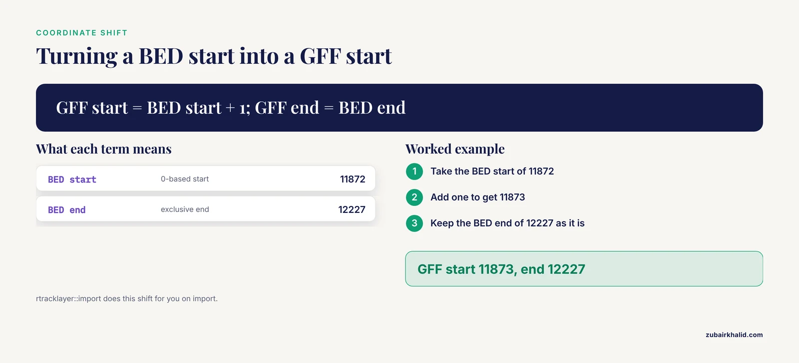
Start with a small BED file called peaks.bed containing three ChIP-seq style peaks. Remember that BED has no header:
chr1    11872   12227   peak_1  250     +
chr1    12721   12795   peak_2  410     -
chr2    28835   29120   peak_3  900     +
Read it into a GRanges and inspect it:
gr <- import("peaks.bed", format = "bed")
gr
Expected output:
GRanges object with 3 ranges and 2 metadata columns:
    seqnames    ranges strand |      name     score
       <Rle> <IRanges>  <Rle> | <factor> <numeric>
  1     chr1 11873-12227      + |    peak_1       250
  2     chr1 12721-12795      - |    peak_2       410
  3     chr2 28835-29120      + |    peak_3       900
Look closely at the ranges. The BED start coordinate 11872 became 11873. rtracklayer performed the 0-based to 1-based shift during import, which is exactly what you want. If you had read the file with read.table instead, the coordinates would still be 0-based and every downstream interval would be off by one.
Add a type column, because GFF3 requires a type for every feature, and export:
gr$type <- "biological_region"
export(gr, "peaks.gff3", format = "gff3")
The output file peaks.gff3 looks like this:
##gff-version 3
chr1    rtracklayer    biological_region    11873    12227    250    +    .    Name=peak_1
chr1    rtracklayer    biological_region    12721    12795    410    -    .    Name=peak_2
chr2    rtracklayer    biological_region    28835    29120    900    +    .    Name=peak_3
The BED name column became the GFF3 Name attribute, the score carried over, and the strand was preserved. Notice the start coordinates. BED 11872 became GFF 11873, a one base shift that is correct, not a bug.
A few parameters matter here. The format argument can be omitted when the file extension is unambiguous, but stating it explicitly makes scripts easier to debug. The genome argument on import attaches a genome identifier to the object, for example import("peaks.bed", genome = "hg38"), and that identifier travels with the object into the exported file metadata where the format supports it. The colnames argument lets you rename metadata columns during import if your BED file uses nonstandard column 4 and 5 content.
Step 3: GFF3 or GTF to BED
Going the other direction, read a GFF3 annotation and export BED:
genes <- import("genes.gff3", format = "gff3")
genes_bed <- genes[, c("ID", "score")]
export(genes_bed, "genes.bed", format = "bed")
Selecting columns with genes[, c("ID", "score")] controls which metadata columns get written. If you export the full object, rtracklayer packs every metadata column it can into the optional BED fields and may warn about columns that do not fit.
GTF files are the more common real-world case, and they deserve a careful walkthrough. A line from an Ensembl or GENCODE style GTF looks like this:
chr7 Ensembl exon 55086742 55086836 . + . gene_id "ENSG00000002587"; transcript_id "ENST00000003100";Try the rtracklayer route first, since recent versions of the package read GTF through the same GFF infrastructure:
gtf <- import("genes.gtf", format = "gtf")
head(mcols(gtf))
You should see metadata columns including type, gene_id, and transcript_id. If your GTF is nonstandard or the import fails, parse it manually. The manual route is also much faster on very large files:
gtf <- fread(
    "genes.gtf",
    header = FALSE,
    sep = "\t",
    col.names = c("seqid", "source", "type", "start", "end",
                  "score", "strand", "frame", "attr"),
    quote = ""
)

gene_id <- sub('.*gene_id "([^"]+)".*', "\\1", gtf$attr)

bed <- data.frame(
    chrom  = gtf$seqid,
    start  = gtf$start - 1L,
    end    = gtf$end,
    name   = gene_id,
    score  = 0,
    strand = gtf$strand
)

fwrite(bed, "genes.bed", sep = "\t", col.names = FALSE)
Three details in that block deserve explanation:
start = gtf$start - 1Lperforms the 1-based to 0-based conversion. The integer suffixLkeeps the column as an integer, which matters for files with millions of rows.quote = ""tellsfreadto treat double quotes as ordinary characters inside the attributes column. Without it,freadcan misparse GTF rows because the attribute field contains unbalanced looking quote characters.col.names = FALSEon write suppresses a header, because BED files have none.
The result is a standard six column BED file. If you want to keep only exons, filter first with gtf <- gtf[gtf$type == "exon"] after the fread call.
Step 4: VCF to BED
Converting a VCF to BED is the most frequent request, because interval tools such as peak overlap functions and liftOver chains all consume BED. Use VariantAnnotation:
vcf <- readVcf("variants.vcf.gz", genome = "hg38")
gr  <- rowRanges(vcf)
gr
Expected output for a small file:
GRanges object with 3 ranges and 4 metadata columns:
    seqnames    ranges strand |        REF        ALT      QUAL      FILTER
       <Rle> <IRanges>  <Rle> | <DNAString> <DNAStringSet> <numeric> <character>
  1     chr1   69511-69511      * |           G              A       285         PASS
  2     chr1 877916-877916      * |           C              T       105         PASS
  3     chr2  89504-89504      * |           A              T        67         PASS
rowRanges(vcf) keeps REF, ALT, QUAL, and FILTER as metadata, while granges(vcf) returns positions only. For a BED of variant positions, the BED start is the VCF POS minus one:
bed <- data.frame(
    chrom = as.character(seqnames(gr)),
    start = start(gr) - 1L,
    end   = end(gr),
    name  = paste0(as.character(seqnames(gr)), "_", start(gr)),
    score = 0,
    strand = "*"
)

fwrite(bed, "variants.bed", sep = "\t", col.names = FALSE)
Output:
chr1    69510   69511   chr1_69511   0   *
chr1    877915  877916  chr1_877916  0   *
chr2    89503   89504   chr2_89504   0   *
One subtlety with indels. In VCF, an insertion at position 100 with REF A and ALT ATTT is anchored at the base before the inserted sequence. The range you get from rowRanges is that single anchor base. If your downstream tool needs the full inserted sequence represented, you must extend the interval yourself, for example with end(gr) <- end(gr) + width(gr$ALT) - 1L after filtering to insertions. Deletions behave differently again, since the REF spans the deleted bases and the range already covers them. Decide what your downstream tool expects before writing the BED, because there is no single correct representation of a VCF indel in BED.
For large whole-genome VCFs, do not read everything into memory. Index the file with tabix, then stream regions:
region <- GRanges("chr7", IRanges(55000000, 56000000))
vcf_slice <- readVcf(TabixFile("variants.vcf.gz"), genome = "hg38",
                     param = region)
readVcf with a GRanges parameter reads only the overlapping records, which turns a multi-gigabyte file into a tractable slice.
Step 5: BED to VCF
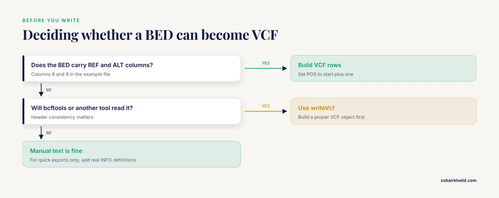
Going from BED to VCF is the reverse direction, and it comes with a structural limitation you must understand before writing code. A VCF row describes alleles, so it needs REF and ALT sequences, a quality score, and filter status. A BED file carries positions only. The conversion is only meaningful when your BED has extra columns holding REF and ALT, for example a file produced from a variant database export:
chr1    69510   69511   rs2236725   .   +   G   A
chr1    877915  877916  rs2845364   .   +   C   T
Columns 8 and 9 here are REF and ALT. Read the file explicitly, then build the VCF text:
snv <- fread(
    "snvs.bed",
    header = FALSE,
    col.names = c("chrom", "start", "end", "id",
                  "qual", "strand", "ref", "alt"),
    colClasses = c("character", "integer", "integer", "character",
                   "character", "character", "character", "character")
)

out <- data.frame(
    CHROM  = snv$chrom,
    POS    = snv$start + 1L,
    ID     = snv$id,
    REF    = snv$ref,
    ALT    = snv$alt,
    QUAL   = snv$qual,
    FILTER = "PASS",
    INFO   = "."
)

header <- c(
    "##fileformat=VCFv4.2",
    "##source=converted_from_bed_in_r",
    paste0("#CHROM\tPOS\tID\tREF\tALT\tQUAL\tFILTER\tINFO")
)

writeLines(header, "snvs.vcf")
fwrite(out, "snvs.vcf", sep = "\t", quote = FALSE,
       col.names = FALSE, append = TRUE)
Note the POS = snv$start + 1L, which reverses the BED offset. The output file:
##fileformat=VCFv4.2
##source=converted_from_bed_in_r
#CHROM	POS	ID	REF	ALT	QUAL	FILTER	INFO
chr1	69511	rs2236725	G	A	.	PASS	.
chr1	877916	rs2845364	C	T	.	PASS	.
The + 1L here and the - 1L in the previous section are the two places where the entire off-by-one battle is won or lost. The VCF specification, maintained in the hts-specs repository used by samtools and htslib, defines POS as the 1-based position of the first base in REF.
For serious pipelines, prefer VariantAnnotation::writeVcf with a properly constructed VCF object over manual text output, because writeVcf enforces header consistency and produces a file that tools like bcftools accept without complaint. The manual route above is fine for quick exports, but add real INFO field definitions in the header if any downstream tool needs them.
Step 6: Fix Chromosome Naming Mismatches
The second most common conversion failure has nothing to do with coordinates. UCSC files use names like chr1, while Ensembl, GENCODE, and NCBI RefSeq-based annotations use 1. When you convert a BED from UCSC into a GTF from Ensembl, every overlap operation returns zero results and nothing warns you.
Check what you have:
table(seqnames(gr))
head(seqlevels(gr))
The cleanest fix for well-known systems is seqlevelsStyle from GenomeInfoDb:
seqlevelsStyle(gr) <- "Ensembl"That single line renames chr1 to 1, chrM to MT, and so on for supported organisms. It throws an error like matched multiple styles when chromosome names are ambiguous, which happens with mixed or unusual assemblies. In that case, rename manually:
mapping <- setNames(
    sub("^chr", "", seqlevels(gr)),
    seqlevels(gr)
)
gr <- renameSeqlevels(gr, mapping)
Always fix chromosome names immediately after import, before any conversion or overlap step, and record which convention you settled on in the file name or project notes. A BED named variants_hg38_ucsc.bed saves hours of confusion three months later.
Step 7: Validate the Conversion
Every conversion should end with checks. These take seconds and catch nearly every silent failure:
gr <- import("converted.gff3", format = "gff3")

stopifnot(
    !any(start(gr) < 1L),
    !any(width(gr) <= 0L),
    !any(is.na(seqnames(gr))),
    all(seqnames(gr) %in% paste0("chr", c(1:22, "X", "Y", "M")))
)

summary(width(gr))
table(strand(gr))
length(gr)
Then cross-check against the original file with a line count. For a headerless BED to GFF3 conversion with three metadata columns, the row counts must match exactly:
length(readLines("peaks.bed"))   # 3
length(grep("^[^#]", readLines("peaks.gff3")))   # 3
For VCF validation, the strongest check available in R is reading your own output back in:
check <- readVcf("snvs.vcf", genome = "hg38")
length(check)
identical(as.character(seqnames(rowRanges(check))), out$CHROM)
identical(start(rowRanges(check)), out$POS)
If a file must satisfy external tools, run bcftools view on the output from the command line. bcftools rejects malformed VCFs with a specific line number, which turns a vague format problem into a one line fix.
Also confirm the genome build survived. Check genome(gr) after import and before export. A BED converted from hg38 coordinates and exported without genome metadata, then later overlapped with an hg19 annotation, produces plausible-looking but completely wrong results, and nothing in either file will alert you.
Tips for Reliable Conversions
These practices keep conversions reproducible across months of analysis:
- Treat
GRangesas the hub. Write every pipeline as format to GRanges, transform, GRanges to format. Two well-tested import and export paths beat a pile of direct parsers. - Pass
genomeexplicitly on every import and keep it attached through every transformation. The BioconductorSeqinfoinfrastructure tracks chromosome lengths and circularity, and carrying it prevents merge errors later. - Use
sort(gr)before export whenever a downstream tool requires sorted input, particularly anything that will be bgzipped and tabix indexed. BED itself does not require sorting, but compressed, indexed BED and VCF files do. - Keep intermediate
GRangesobjects withsaveRDS(gr, "step1.rds")so you can rerun the export step without re-reading a 40 GB VCF. - For files over a few hundred megabytes, prefer
freadoverread.tablefor manual parsing, and prefer region-constrainedreadVcfover whole-file reads for variants. Reading a whole genome VCF without a param can exhaust memory on a typical laptop. - Record the exact version of
rtracklayerandVariantAnnotationin your analysis log withpackageVersion("rtracklayer"). GTF parsing behavior has changed across package versions, and reproducibility depends on knowing which one you used.
Common Mistakes and Limitations
The off-by-one error from mixing coordinate systems. BED is 0-based with an exclusive end. GFF3, GTF, and VCF are 1-based with inclusive ends. If you import a BED with read.table instead of rtracklayer::import, or write GFF coordinates with a manual fwrite without adding one to the start, every interval shifts. The symptom is subtle: individual features look fine, but overlaps with other files are off by one base, and short features like single-base peaks lose or gain the wrong base entirely. The fix is to use rtracklayer for both directions or to perform the shift explicitly and exactly once in your own code.
Assuming a header. BED files have no header by definition. Calling fread("file.bed") without header = FALSE consumes the first real interval as column names, and every downstream count is one too small. Conversely, some GTF files distributed with pipelines have been given a header by someone else, and header = FALSE then treats it as data. Check the first lines with readLines("file.bed", n = 3) before choosing the setting.
Losing GTF attributes to parsing errors. The attribute column is a semicolon separated string with embedded double quotes, and naive string splitting breaks on values containing semicolons or on files that omit the trailing semicolon. The regular expression sub('.gene_id "([^"]+)".', "\\1", x) returns the gene_id, but if the file lacks that key it silently returns the whole attribute string as a value. Verify with table(nchar(gene_id)) or a few head() calls before trusting the column.
Expecting one interval per variant for indels. A VCF insertion is anchored to a single base, so converting to BED produces a one base interval even though the inserted sequence can be thousands of bases long. A deletion produces an interval spanning the deleted bases. Treating all variant records as point positions misrepresents indels in any downstream interval analysis.
Mixed chromosome naming. As covered in Step 6, chr1 versus 1 is the most common reason a conversion produces a valid file that yields zero overlaps. Silent zero-result overlaps deserve the same suspicion as hard errors.
Invalid BED score values. The UCSC BED specification defines the score column as an integer from 0 to 1000. GFF score fields are unbounded floats. Exporting a GFF with a score of 3750 to BED and loading it into a genome browser can cause the track to fail to display. Clamp or rescale scores before exporting to BED if the file is destined for UCSC tools.
Windows line endings and UCSC track lines. Files saved on Windows can carry carriage return characters that break strict parsers. Files downloaded from the UCSC Table Browser often begin with browser and track lines. Strip them at import with skip arguments in fread or by reading and filtering lines first. The error invalid start value from rtracklayer is often a hidden carriage return rather than a coordinate problem.
Assumed genome equivalence. Converting a file between formats does not convert it between genome builds. An hg19 BED exported as GFF3 is still hg19 data. Every coordinate transformation across builds requires a dedicated lift-over step with a chain file, which is a separate operation from format conversion.
What conversions cannot do. Format conversion moves positions and whatever metadata you explicitly carry across. It does not create information. A BED converted to VCF has no genotypes, no read depth, and no filter history unless you supply them from another source. A GFF converted to BED keeps only the columns you select. Document what was dropped, because the output file will not tell anyone. And as with any pipeline step, verify conversions against the original files on a small sample rather than trusting an error-free run.
Frequently Asked Questions
Can rtracklayer write VCF files directly?
No. rtracklayer reads and writes BED, GFF, GTF, WIG, and BigWig, but VCF input and output belong to the VariantAnnotation package. Use readVcf and writeVcf for VCF work, or write simple VCF text manually as shown in Step 5.
Why are my intervals shifted by one base after converting BED to GFF?
BED uses 0-based start coordinates and GFF uses 1-based coordinates. If the shift appears after a conversion, the 0-to-1 adjustment was either applied twice or not at all. Use rtracklayer::import and export for both formats and let the packages handle the offset, or apply the shift manually exactly once.
How do I convert an Ensembl GTF to a BED file?
Import with rtracklayer::import("genes.gtf", format = "gtf") and export with export(gr, "out.bed", format = "bed"), or parse the nine columns with fread and subtract one from every start coordinate. Extract the gene or transcript identifier from the attributes column with a regular expression before writing.
What is the difference between GFF3 and GTF?
Both are nine column, 1-based formats. GFF3 attributes use key equals value pairs with percent encoding and support a full feature hierarchy through Parent relations. GTF attributes use quoted key value pairs and is the convention used by Ensembl and GENCODE gene annotation releases. For R code, rtracklayer reads both, and GFF3 round trips metadata more faithfully.
How do I convert a large VCF file without running out of memory?
Index the VCF with tabix and read it in slices using readVcf(TabixFile("file.vcf.gz"), genome = "hg38", param = my_granges). Process and write each slice before reading the next. Reading a whole genome VCF into a single object routinely needs far more RAM than the file size suggests.
Can I convert BED to VCF?
Only if the BED file carries REF and ALT sequences in extra columns, because VCF rows describe alleles, not just positions. Construct the VCF text with the eight fixed fields, add the required ## header lines, and shift BED starts up by one to get VCF positions. A BED without allele information cannot become a meaningful VCF.
How do I fix chromosome name mismatches like chr1 versus 1?
Use seqlevelsStyle(gr) <- "Ensembl" or seqlevelsStyle(gr) <- "UCSC" from GenomeInfoDb for standard organisms, or renameSeqlevels with a named character vector when names are ambiguous. Do this immediately after import, before any overlap or export step.
Do I need Bioconductor for this or can base R handle the conversions?
Base R can read and write any of these files with read.table and write.table, and for tiny files that is workable. You would have to manage coordinate shifts, headers, attribute parsing, and chromosome naming yourself. Bioconductor packages do all of that correctly and are tested against the format specifications, so for anything beyond a quick one-off they are the right tool.