How to Compare Genome Assemblies on NCBI
By Dr. Zubair Khalid, DVM, MS, PhD ·

Comparing genome assemblies is a critical task in comparative genomics. It allows researchers to identify large structural changes, pinpoint functional divergence, and assess the quality of sequencing efforts across different species or strains. The fundamental difference between comparison methods lies in the scope of the analysis. Global structural comparison looks at the entire chromosome structure and large-scale rearrangements. Local or annotation comparison focuses on the specific location and sequence of genes, coding regions, and functional elements. The rule of thumb is to start with a global visualization tool like the Comparative Genome Viewer (CGV) to identify major structural events before diving into detailed gene-level comparisons using annotation-specific tools.
Core Methods for Comparing Genome Assemblies on NCBI
NCBI provides several powerful resources for comparing genome assemblies. The choice of tool depends entirely on the research question. Do you want to see if two chromosomes have been inverted? Use a visualization tool. Do you want to know if a specific gene has been gained or lost? Use annotation comparison tools. Do you want to verify if the predicted protein is actually present? Use proteomic validation methods.
Global Structural Comparison using the Comparative Genome Viewer (CGV)
The NCBI Comparative Genome Viewer (CGV) is the primary tool for visualizing whole-genome assembly alignments [1][8]. This platform is designed to help researchers examine pairwise alignments between two different assemblies, whether they are from the same species (intraspecies comparison) or different species (cross-species comparison). CGV uses sophisticated assembly alignment algorithms to generate visualizations of large structural differences [1][8].
How CGV Works
When you use CGV, you are typically comparing two reference genomes. The tool allows you to view these alignments in two main formats:
- The Ideogram-Based View: This view presents the chromosomes as a linear or circular map, similar to a traditional karyotype. It displays the overall structure and allows you to navigate to specific regions of interest. If gene annotation (like RefSeq or user-provided annotation) is available, it is displayed within this view [1][8]. This is excellent for quickly assessing chromosome organization.
- The 2D Genome Dotplot: This view is a matrix visualization where the axes represent the coordinates of the two compared genomes. A diagonal line or cluster of dots indicates regions of high sequence similarity. Off-diagonal dots or breaks in the diagonal line reveal large-scale structural events. For example, a sudden shift in the dot pattern can signal a translocation or a large insertion.
Identifying Structural Differences
CGV is particularly powerful for detecting major evolutionary events. Researchers can use this tool to expose large structural differences spanning entire chromosomes, such as inversions or translocations [1]. By examining the alignment plots, you can visually confirm whether two genomic regions have been flipped or moved relative to each other.
For instance, if you compare two assemblies and observe a significant break in the diagonal dotplot followed by a sudden jump in the sequence correspondence, this strongly suggests a large-scale chromosomal rearrangement has occurred between the two organisms.
Functional and Annotation Comparison
While CGV excels at showing where the pieces are, it does not inherently tell you if the parts (the genes) are correct or if they have changed function. This requires tools that compare the annotations, which are the functional descriptions of the sequences.
Comparing Gene Annotations with CDScompare
The rapid proliferation of high-quality genome assemblies means that we often have multiple annotation sources for a single genome. These sources can include predictions from dedicated pipelines, manually curated data, or public repositories like NCBI [1]. The challenge is that these different sources might conflict.
CDScompare is a specific tool designed to address this problem by performing frame-sensitive comparison of GFF (General Feature Format) annotation files [1].
The Importance of Frame Sensitivity
A gene is a sequence of DNA that contains instructions for making a protein. This protein is coded in specific segments called coding sequences (CDS). The reading frame is the way the genetic code is read, usually three nucleotides at a time. If a tool compares two sequences without considering the reading frame, it might flag a difference that is actually irrelevant. However, if a single nucleotide changes and shifts the reading frame, it can completely change the resulting protein.
CDScompare accounts for this crucial detail. It is a Python-based tool that focuses on detecting differences in coding/non-coding boundaries, gene overlaps, fusions, or splits, while ensuring that the comparison is done in a frame-aware manner [1]. This is vital for accurately identifying functionally relevant annotation conflicts.
Relying on Standard Pipelines (PGAP)
For large-scale, automated annotation, NCBI provides the Prokaryotic Genome Annotation Pipeline (PGAP) [7]. PGAP is a comprehensive framework that combines alignment-based methods with predictive tools to generate and modify gene predictions across the entire genome. When you use PGAP, you are relying on a robust, standardized process that utilizes sequence similarity and statistical predictions to assign functions to genes [2].
When comparing two genomes, using PGAP provides a consistent baseline annotation. However, if you are comparing a PGAP-derived annotation against a manually curated annotation, you must use a tool like CDScompare to resolve discrepancies accurately [1].
Validation and Quality Metrics
The best assembly is one that accurately reflects biological reality. Sometimes, the best way to compare two assemblies is not with a bioinformatics tool, but with a biological measurement.
Proteomic Validation
Proteomics is the study of proteins. By performing mass spectrometry on biological samples derived from the organisms whose genomes you are studying, you can identify the actual proteins present [3]. Comparing the list of predicted proteins from your genome annotation against the list of actual proteins identified by mass spectrometry provides a powerful validation metric.
For example, one metric proposed is NP10, which measures the quality of annotation by looking at the median molecular weight of the top decile of identified proteins based on the number of peptides per protein [3]. A higher NP10 score suggests a higher quality and more accurate genome annotation because it indicates that the predicted genes are being correctly translated into stable, identifiable proteins [3].
Side-by-Side Comparison of Genome Comparison Tools
| Comparison Goal | Primary Tool / Method | Scope of Analysis | What it Detect | Pros | Cons |
|---|---|---|---|---|---|
| Structural Rearrangements | NCBI Comparative Genome Viewer (CGV) | Whole Genome / Global | Inversions, translocations, large insertions, chromosomal shifts. | Highly visual, interactive, excellent for large-scale changes [1][8]. | Does not assess gene function, requires pre-existing alignments. |
| Annotation Conflict Resolution | CDScompare | Local / Gene-Specific | Gene overlaps, fusions, splits, frame-sensitive coding discrepancies. | Frame-aware, highly precise for annotation comparison [1]. | Requires pre-existing GFF annotation files, not a whole genome comparison tool. |
| Automated Gene Identification | PGAP (NCBI Pipeline) | Whole Genome / Automated | Gene prediction, functional assignment based on homology and prediction [2]. | Standardized, scalable, provides a consistent reference annotation [2]. | Relies on algorithms and database similarity, may miss novel or highly divergent genes. |
| Annotation Quality Validation | Proteomics / NP10 Metric | Phenotypic / Global | Accuracy of predicted protein sequences and gene models. | Measures biological reality, provides a hard metric for quality [3]. | Requires access to biological samples and expensive mass spectrometry equipment. |
Detailed Workflow Scenarios
Scenario 1: Investigating Evolutionary Divergence Between Two Species
Research Question: Have two closely related plant species undergone significant chromosomal rearrangements since their divergence?
Workflow:
- Data Acquisition: Obtain the RefSeq assemblies for both species from NCBI.
- Tool Selection: Use the NCBI Comparative Genome Viewer (CGV) [1][8].
- Execution: Upload or select the two assemblies within the CGV interface.
- Analysis:
- Examine the ideogram view first to confirm that the overall chromosome number and size are similar.
- Zoom into the 2D dotplot. Look for sudden breaks or shifts in the alignment pattern.
- If you see a clear breakpoint in the dotplot, this indicates a potential translocation or large deletion.
- Refinement: Navigate to the region of interest in the ideogram view. Check the displayed gene annotations to see if the genes on either side of the breakpoint are conserved or if they have been disrupted [1][8].
Scenario 2: Resolving Conflicting Gene Predictions
Research Question: A study used two different annotation pipelines for the same bacterial genome and found conflicting predictions for a key metabolic gene. Which prediction is more likely correct?
Workflow:
- Data Acquisition: Obtain the GFF annotation files for both versions of the genome assembly.
- Tool Selection: Use CDScompare [1].
- Execution: Run the CDScompare tool, providing the two GFF files as input.
- Analysis:
- CDScompare will compare the CDS regions of the conflicting gene.
- It will specifically flag whether the predicted coding sequences overlap, are split, or if the difference lies in the reading frame.
- If one prediction maintains the reading frame and the other does not, the prediction that respects the frame is likely the functionally correct one, assuming the underlying sequence is correct [1].
Scenario 3: Analyzing Functional Differences in Gene Sets
Research Question: How do the functional gene repertoires of bacteria adapted to leaf environments differ from those adapted to soil environments?
Workflow:
- Data Acquisition: Download the complete genomic sequences for the leaf-associated (LA) and soil-associated (SA) bacterial strains from NCBI.
- Annotation: Use the NCBI Prokaryotic Genome Annotation Pipeline (PGAP) to generate standardized functional annotations for all strains [7].
- Functional Analysis: Use sequence comparison tools (like BLAST) against large databases such as the NCBI Nonredundant (NR) protein sequence database [2].
- Interpretation: Compare the enrichment of specific functional categories. For example, if LA strains show significantly higher enrichment for genes related to cell wall degradation compared to SA strains, this suggests a functional adaptation to the plant leaf environment [4].
Advanced Comparative Genomics and Specific Use Cases
Beyond general structure and function, genome comparison is used for highly specialized tasks.
Phylogenetic Reconstruction and Taxonomy
When comparing mitochondrial genomes, researchers can reconstruct phylogenetic relationships to understand evolutionary history [5]. By collecting mitochondrial genome sequences from multiple species in a specific family, such as Carabidae, and feeding them into phylogenetic analysis tools, one can map the evolutionary distance between subfamilies [5]. This process uses sequence similarity to build a tree of life for that group.
Analyzing Mobile Genetic Elements (TEs)
Transposable elements (TEs) are mobile genetic elements that can jump around a genome, significantly impacting its structure and function [6]. When comparing assemblies, accurately annotating TEs is vital because they often constitute a large portion of the genome [6].
The annotation of TEs can be challenging, especially as the phylogenetic distance between the queried genome and the reference increases [6]. Researchers must use multiple methods, including homology-based searching and de novo (from scratch) assembly methods, and often require manual curation to ensure complete TE annotation [6].
Comparative Functional Enrichment
Comparative functional analysis allows researchers to identify genes that are conserved (present in all strains) versus genes that are unique or highly enriched in specific ecological niches [4]. By comparing the functional gene profiles of different microbial populations, scientists can infer the ecological adaptations of those organisms.
For instance, analysis of specific bacteria has shown that certain genes like cytochrome P450 or DNA repair are significantly enriched in strains adapted to leaf environments, suggesting a specific functional role in environmental adaptation [4].
Common Mistakes and Limitations
When comparing genome assemblies, errors can arise from the data itself or from the interpretation of the tools.
Misinterpreting Assembly Quality: A structural difference detected by CGV might not be a biological event. It could be an artifact of the assembly process, where the assembler incorrectly ordered contigs. Always cross-reference structural changes with known biological mechanisms before concluding a rearrangement occurred.
Ignoring the Reading Frame: The most common mistake when comparing annotations is failing to use frame-sensitive tools like CDScompare. Comparing raw nucleotide sequences without accounting for the reading frame will yield false positives, leading to incorrect conclusions about gene structure [1].
Assuming Completeness: Even the most advanced pipelines like PGAP are probabilistic. They rely on statistical likelihood and homology. A genome annotation is a best-guess model, not a perfect map. Always validate critical findings, especially gene presence or absence, using external data like proteomics [3].
Database Limitations: When using comparative tools, the quality of the output depends entirely on the quality of the input databases. If the reference database used for functional annotation is outdated or incomplete, your comparison results will be limited, regardless of how good your comparison tool is [7].
Preparing Your Data Before You Compare Anything
Most failed assembly comparisons fail before the analysis even starts, and they fail for boring reasons: mismatched assembly versions, incompatible file formats, or assemblies downloaded from different sources at different times. A short preparation phase saves hours of confusion later, and it makes your comparison reproducible for anyone who reads your work.
Understanding Assembly Accessions and Versions
Every assembly in the NCBI Assembly database carries two identifiers when both records exist: a GenBank accession beginning with GCA and a RefSeq accession beginning with GCF. These are not interchangeable. The GenBank record is the submitter-provided assembly, while the RefSeq record has passed through NCBI's curation, which can include contig renaming, filtering, and coordinate changes. When you select two assemblies inside the Comparative Genome Viewer (CGV), you should always check which accession you are actually viewing [1][8].
Two practical rules follow from this:
- Compare like with like. If you compare a GenBank assembly of species A against a RefSeq assembly of species B, part of any structural difference you observe may come from curation rather than biology. Prefer either both GenBank or both RefSeq versions when the goal is evolutionary inference.
- Record the version number. Assemblies are updated. An assembly you compared six months ago may have been replaced by a newer patch release, and CGV will happily show you the current version, which may not be the one your earlier screenshots came from. Note the full accession, including version suffix, in your lab notebook or methods section.
Assembly Level Matters More Than Most Beginners Realize
The Assembly database labels each entry as Contig, Scaffold, or Chromosome level. This label describes how far the assembly process progressed. A contig-level assembly is a set of unordered fragments, which makes global comparison nearly meaningless because there is no chromosome-scale structure to compare. A chromosome-level assembly places sequences onto chromosomes, which is the minimum input for a sensible dotplot or ideogram comparison.
Before starting a structural comparison in CGV, open each assembly's record page and confirm:
- The assembly level is at least scaffold, and ideally chromosome.
- The assembly has a molecular map or chromosome assignment, so sequences can be displayed in order.
- The statistics (total length, number of contigs, N50) are broadly comparable between the two assemblies.
If one assembly has two hundred contigs and the other has twelve chromosomes, any comparison you run will mostly reflect the fragmentation gap, not biology. In that situation, either upgrade to a more complete assembly or explicitly frame your comparison as a contig-level one.
Gathering the Right Files
For structural comparison inside NCBI's web tools, you usually only need the accessions. For annotation comparison, you need the underlying files, and the format matters:
- Genomic FASTA: the nucleotide sequence itself. This is the substrate every alignment depends on.
- GFF3 or GenBank feature files: the annotation. PGAP-derived annotations for prokaryotic genomes are distributed in specific standardized formats, and tools like CDScompare depend on properly structured GFF input [5][7].
- Protein FASTA: the translated products of the annotation, useful for downstream BLAST searches against the NCBI Nonredundant protein database [2].
Download the files for both assemblies in a single session, note the download date, and keep directory names that encode the accessions. When two files later produce a confusing result, being able to confirm that both files came from the same download batch and the same assembly version eliminates an entire class of error.
A Note on Coordinate Systems
Genome coordinates are zero-based in some files and one-based in others, and different NCBI tools and file formats handle this differently. When you note a region of interest in CGV and then try to extract the same region from a FASTA file locally, an off-by-one discrepancy is common. Always confirm the coordinate convention of the tool or file you are working with before extracting sequences, and when reporting a region to colleagues, state which assembly and which coordinate system the numbers refer to.
A Guided Walkthrough of the Comparative Genome Viewer
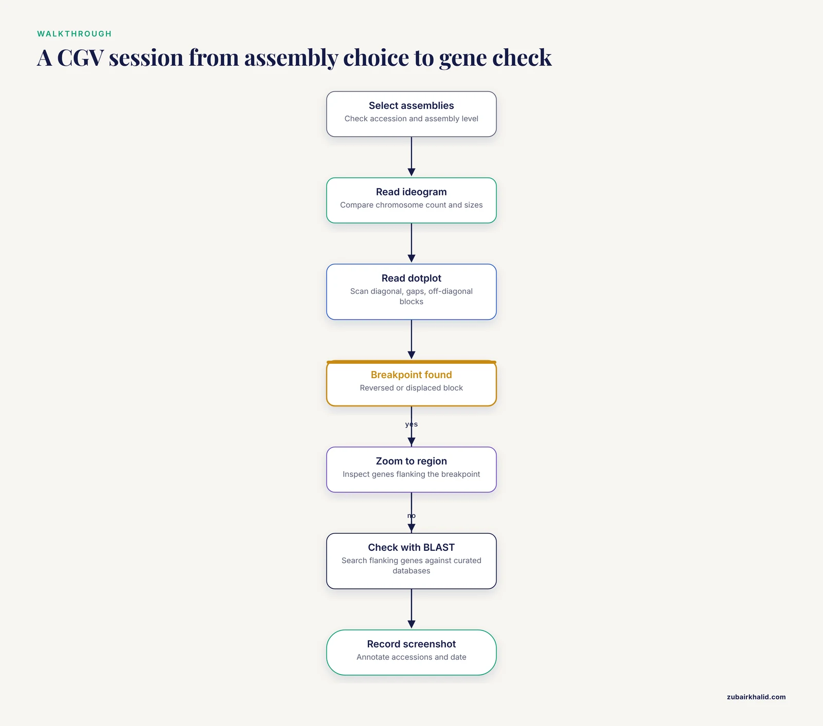
The Comparative Genome Viewer is the recommended entry point for assembly comparison because it requires no local installation and it aligns assemblies for you rather than expecting precomputed alignment files [1][8]. Here is a detailed walkthrough of a typical session, written as you would actually experience it.
Step 1: Selecting the Assemblies
Begin by choosing the two assemblies. CGV supports comparisons between assemblies of the same species and between assemblies of different species [1]. In practice, you select the assemblies through the interface by searching for organisms or accessions.
When selecting, pay attention to three things:
- Both assemblies should be at a comparable level of completeness, as discussed above.
- One assembly should ideally be a well-characterized reference. Comparing a draft assembly against a curated reference is the most common and most interpretable use case.
- If you are comparing within a species, note the source strain or isolate of each assembly, because intraspecies structural variation is real and common in many groups.
Step 2: Starting with the Ideogram View
The ideogram view presents chromosomes as structured maps, similar in spirit to a karyotype, and displays gene annotation where it is available [1][8]. Resist the temptation to jump straight to the dotplot. The ideogram answers framing questions first:
- Do the two assemblies have the same chromosome count?
- Are chromosome sizes broadly similar?
- Are there sequences in one assembly that have no chromosome assignment at all?
If the chromosome counts differ, that observation shapes everything that follows. A missing chromosome might mean a genuine biological difference, an unplaced scaffold set in one assembly, or a different treatment of organellar sequences. The ideogram lets you see this in seconds.
Step 3: Moving to the Dotplot for Detail
Switch to the two-dimensional dotplot view. Each axis represents the coordinate space of one assembly, and aligned blocks appear as marks. In an ideal comparison of two identical assemblies, you would see a clean diagonal. In real comparisons, you see a diagonal assembled from segments, with breaks, offsets, and occasionally reversed segments.
A disciplined reading order for the dotplot:
- Scan the overall diagonal first. Does the large-scale diagonal run from the lower-left to the upper-right of the plot? If large segments run in the opposite orientation, those are candidates for inversions.
- Look for long stretches with no aligned blocks. These gaps suggest sequence present in one assembly and absent from the other, which may be an insertion, a deletion, or sequence that simply failed to align.
- Look for segments that sit far off the diagonal. An aligned block that appears in an unexpected part of the plot is a candidate translocation, meaning a piece of one chromosome matches a different chromosome in the other assembly.
- Note repeated blocks appearing more than once. Segmental duplications or repetitive elements can produce multiple alignment blocks for the same region.
Step 4: Zooming In and Cross-Referencing Genes
When you identify a region of interest, navigate to it in the ideogram view and inspect the gene content on either side of the apparent breakpoint [1]. Two genes flanking a breakpoint in one assembly, separated by unrelated sequence in the other, is strong visual evidence of a rearrangement. Genes that are intact on one side and truncated on the other deserve follow-up at the sequence level with BLAST against curated protein databases [2].
Troubleshooting Common CGV Problems
The dotplot is mostly empty. This usually means the two assemblies are too divergent for whole-genome alignment to find many blocks, or one assembly is heavily fragmented. Check the assembly levels first. Cross-species comparisons at large evolutionary distances will naturally show sparse alignment.
Alignments exist but the chromosomes seem mismatched. Different assemblies name and order chromosomes differently, particularly when one is GenBank and the other is RefSeq. A chromosome called by number in one assembly may be called differently in the other. Visual alignment blocks are the reliable guide, not the labels.
A "rearrangement" appears exactly at a contig boundary. This is the classic fragmentation artifact. If a suspicious breakpoint falls at the end of a contig or scaffold, treat it as unproven until validated by an independent method. Assemblers can misjoin or misorder sequences, and CGV will faithfully display whatever the assemblies say, including their errors.
The plot is unreadably dense. Very repeat-rich or very large genomes produce crowded plots. Zoom into a single chromosome pair rather than viewing everything at once, and work chromosome by chromosome.
Interpreting Dotplot Patterns: A Working Visual Dictionary
Because the dotplot is the single most information-dense view in CGV, it deserves its own interpretation guide. The patterns below cover the situations most researchers encounter.
A clean, continuous diagonal. The two assemblies agree in both sequence and order across the region. Little to report structurally, which is itself a finding when comparing divergent isolates.
A diagonal with a reversed segment. A block that runs anti-parallel to the main diagonal, flanked by regions that remain parallel, is the signature of an inversion. The endpoints of the reversed block are your inversion breakpoints, and those breakpoints are worth examining at the gene level because inversions can disrupt or rewire genes at their edges.
A diagonal that jumps sideways. If the aligned blocks continue with the same orientation but shift to a different position along one axis, the intervening sequence has been inserted, deleted, or relocated. A sideways jump between different chromosomes in the ideogram view indicates a translocation.
A staircase of short blocks. Many short parallel blocks stepping across the plot usually indicate one assembly is more fragmented than the other. The underlying sequence may be identical; the ordering information is simply missing in the draft assembly. Do not report a series of rearrangements when the real explanation is fragmentation.
Scattered isolated dots with no diagonal. This suggests only short or sparse similarity, typical of distant organisms, heavily repetitive sequence, or assemblies of poor quality. Whole-genome structural comparison may not be the right approach at this divergence level; targeted gene-by-gene comparison is more informative.
Symmetric mirrored patterns. Complex mirror-image structures can indicate duplicated regions or more complex rearrangement histories involving multiple events. These require careful, often locus-by-locus analysis and should be described conservatively in publications.
A useful habit is to take screenshots of every region you intend to cite. CGV is an interactive web tool, so the exact view you analyzed exists only in your session unless you capture it [8]. Annotate your screenshots with the assembly accessions and the date.
Running an Annotation Comparison in Practice
Structural comparison tells you where sequence sits. Annotation comparison tells you what the sequence is claimed to do. These are different questions, and the second one is where many projects hit trouble, because annotations from different sources disagree more often than beginners expect [1].
Why Annotations Disagree
Three sources of disagreement dominate:
- Different pipelines make different predictions. Gene predictors balance sensitivity against specificity, and different tools land in different places. A gene split into two models by one pipeline may be fused into one model by another.
- Different starting sequence. If the two annotations were built on different assemblies of the same organism, every downstream difference mixes assembly error with annotation error.
- Different evidence and curation levels. A manually curated annotation and an automated prediction are not peers. When they conflict, the curated annotation carries more weight, but it still deserves verification rather than blind acceptance.
What Frame Sensitivity Means in a Real Comparison
Consider a concrete example. Suppose two annotation versions describe a metabolic gene. Version A predicts a single coding sequence of, say, moderate length. Version B predicts two shorter coding sequences in the same interval. A naive comparison would report "one gene versus two genes" and stop there.
A frame-aware comparison asks sharper questions [1]:
- Do the two short coding sequences in version B together cover the same coding span as the single sequence in version A?
- Is each predicted reading frame intact, or does one version contain a frameshift relative to the other?
- Does one version's prediction overlap an adjacent gene, and does the other version's prediction avoid that overlap?
These distinctions matter biologically. A frameshift turns a functional protein prediction into a pseudogene-like fragment. An overlap may indicate an operon context or an annotation error. A fusion or split changes the protein product count, which changes every downstream analysis that counts genes [1].
A Step-by-Step CDScompare Workflow
CDScompare is a Python-based tool that performs frame-sensitive comparison of GFF annotation files, focusing on coding and non-coding boundary differences, gene overlaps, fusions, and splits [1]. A practical workflow looks like this:
- Collect both GFF files and confirm they refer to the same underlying sequence. If the two annotations were built on different assemblies, record that fact, because it changes interpretation.
- Verify format consistency. GFF files come in flavors, and attributes can be structured differently by different pipelines. Confirm that feature types are labeled as expected, with CDS features present and correctly parented to their genes.
- Run the comparison. Provide the two GFF files as input to the tool and let it perform the frame-aware comparison of coding features [1].
- Triage the output by category. Differences in coding versus non-coding boundaries, overlaps, fusions, and splits each carry different implications. Boundary shifts may reflect start or stop codon choice differences. Fusions and splits change gene counts. Overlaps may be real biology or annotation error.
- Validate flagged cases individually. For each important discrepancy, extract the relevant nucleotide region and examine the reading frame directly. Where a protein product is central to your conclusions, search the predicted protein against curated databases with BLAST to see whether an independent hit supports one prediction over the other [2].
The Pitfall of Comparing Annotations Built on Different Assemblies
This deserves its own paragraph because it is a common mistake. If assembly version 1 and assembly version 2 differ, then an annotation difference may simply reflect the assembly difference, not a change in annotation methodology or biological reality. Before attributing an annotation conflict to the pipelines, confirm that the underlying nucleotide sequences of the compared regions are identical. If they are not, the first question is whether the assembly change is real or an artifact, and only then does the annotation comparison become interpretable.
Working with PGAP for Consistent Baseline Annotations
When your comparison involves prokaryotic genomes, the NCBI Prokaryotic Genome Annotation Pipeline provides the standardization that makes cross-assembly annotation comparison meaningful [7]. PGAP combines alignment-based methods with predictive tools, using sequence similarity and statistical models to predict genes and assign functions across a whole genome [2].
Why a Common Pipeline Improves Comparisons
Imagine comparing the gene content of two bacterial strains where one was annotated by pipeline X and the other by pipeline Y. Any difference in gene count could come from biology or from pipeline behavior. Re-annotating both strains with the same pipeline, PGAP, removes the pipeline variable [2]. The remaining gene content differences are then far more likely to reflect the genomes themselves.
This principle extends to functional comparisons. In studies comparing the functional gene repertoires of ecologically distinct bacterial strains, standardized PGAP annotation followed by sequence comparison against large protein databases such as the NCBI Nonredundant database is the recommended path [2][7].
Practical Considerations When Using PGAP
Pipeline versions change. Like assemblies, the annotation pipeline is updated over time. Two genomes annotated years apart under different pipeline versions are not perfectly comparable. Where feasible, annotate all genomes in a study under a single pipeline version, and always record the version.
PGAP output is a model, not a census. The pipeline relies on homology and statistical prediction [2]. Highly divergent or novel genes may be missed, and functions assigned by similarity are only as good as the database hits. Treat PGAP output as a strong hypothesis that critical claims should be validated independently, for example with proteomics.
Standardized output eases downstream work. Because PGAP output follows consistent conventions, downstream comparison tools, including frame-aware annotation comparators, can process it reliably [5][7]. This is a practical reason to prefer it over ad hoc annotation methods when the goal is comparison.
Choosing Between NCBI Comparison Options: A Decision Framework
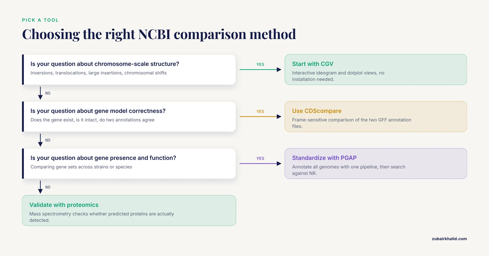
Readers searching for the best way to compare genome assemblies on NCBI usually want a decision procedure, not a tool list. Here is one.
If your question is about chromosome-scale structure (inversions, translocations, large insertions), start with CGV. It is interactive, requires no installation, and displays both ideogram and dotplot views with annotation overlay [1][8].
If your question is about gene model correctness (does this gene exist, is it intact, do two annotations agree), use a frame-sensitive annotation comparator on the relevant GFF files [1], supported by a standardized annotation pipeline for the baseline [2].
If your question is about gene presence, absence, and function across strains or species, standardize annotation with a consistent pipeline, then compare gene sets and functions using sequence similarity searches against comprehensive databases [2][7].
If your question is about whether predicted proteins are real, turn to proteomic validation. Mass spectrometry of biological samples identifies which predicted proteins are actually detected, and metrics such as NP10, which reflects the median molecular weight of the top decile of identified proteins ranked by peptide count, quantify annotation quality [3].
If your question is about evolutionary relationships among many genomes, the comparison shifts from pairwise to phylogenetic. Collecting homologous sequences, for example whole mitochondrial genomes from multiple species, and building trees maps evolutionary distance across the group [5].
The framework's underlying logic: structural questions need alignment views, annotation questions need frame-aware file comparison, functional questions need standardized pipelines plus database searches, and validation questions need independent data such as proteomics [1][5][7][8].
The Pros and Cons in Fuller Detail
The table in the main article summarizes the trade-offs. Here is the reasoning behind each row, expanded.
CGV. Its strengths are accessibility and interpretability. Anyone with a browser can produce a publication-grade visual of two assemblies aligned, and the dual ideogram and dotplot views serve both overview and detail [1][8]. Its limitations follow from its scope: it displays structural relationships but does not evaluate whether annotations are correct, and it depends on the quality of the underlying alignments and assemblies. A fragmented input assembly produces a fragmented and potentially misleading comparison.
CDScompare. Its strength is precision on exactly the question most annotation comparisons get wrong: gene structure at the frame level [1]. Its limitations are that it requires prepared GFF inputs and addresses gene-level questions, not whole-genome structure. It is a scalpel, not a map.
PGAP. Its strengths are standardization and scale: a single consistent annotation framework applied across genomes, which is a precondition for fair comparison [2]. Its limitation is that it is prediction-based; genuinely novel or highly divergent genes can be missed or misassigned, and users must remember that automated functional assignment reflects database similarity, which itself depends on database currency [7].
Proteomic validation. Its strength is independence: mass spectrometry evidence does not care what the predictor predicted, it reports what proteins are detected in the sample, making metrics like NP10 a hard external check on annotation quality [3]. Its limitation is practical: it requires biological material and mass spectrometry access, which puts it out of reach for many projects, and it validates only expressed, detectable proteins, so absence of evidence is not evidence of absence.
Common Misconceptions About Comparing Assemblies
Misconception 1: Two assemblies of the same species should look the same. Intraspecies structural variation is real. Different isolates can carry genuine inversions, insertions, and translocations. At the same time, some differences are assembly artifacts. The comparison cannot by itself tell you which is which; cross-referencing with biology and assembly quality metrics is required.
Misconception 2: The RefSeq annotation is ground truth. RefSeq annotations are curated and far better than raw predictions, but curation is still a model-building exercise. When a curated annotation and experimental evidence conflict, the evidence wins.
Misconception 3: A break in the dotplot diagonal proves a rearrangement. A dotplot break proves the alignments say something changed. It could be a real rearrangement, an assembly error, a difference in how repeats were resolved, or a gap in one assembly. Dotplots generate hypotheses; independent validation confirms them.
Misconception 4: Similar alignment means orthologous function. Two regions that align well are similar in sequence. Function can diverge without much sequence change, and similarity hits against the Nonredundant database are a starting point for functional inference, not a conclusion [2]. Frame-aware annotation comparison and functional enrichment analysis add the necessary layers [2][5].
Misconception 5: More detected differences mean a worse assembly. Sometimes a more complete assembly reveals differences that a worse assembly hid. Comparing a highly fragmented assembly against a chromosome-scale one will show many apparent changes, most of which reflect fragmentation. Assess assembly statistics before interpreting the comparison.
Misconception 6: Transposable element annotations are complete by default. TE annotation is genuinely hard, and its difficulty grows with the evolutionary distance between the genome of interest and available references. Homology-based methods miss elements absent from reference libraries, and de novo methods produce false positives. Complete TE characterization typically requires combining methods with manual curation, a fact that directly affects any comparison involving repeat-rich genomes [6].
A Troubleshooting Guide for Assembly Comparison Projects
The following catalogue pairs symptoms with likely causes and fixes, drawn from the recurring failure modes of comparative assembly work.
Symptom: The dotplot shows a massive offset that no literature supports. Likely causes: assembly error, wrong assembly version loaded, or a chromosome naming and ordering mismatch between the two assemblies. Fix: confirm accessions and versions, check the assembly statistics for both, and verify the region with sequence-level search such as BLAST before believing the offset [2].
Symptom: Annotation comparison reports hundreds of differences between two versions of one genome. Likely causes: the two GFF files were built on different assemblies, or the files use different formatting conventions that the comparator misreads. Fix: confirm that both annotations were built on identical sequence. If they were, check that feature types and parent-child relationships in the GFF files are well formed before trusting the output [1].
Symptom: A key gene appears in one annotation but not the other. Likely causes: a frameshift in one assembly version, a genuine presence-absence difference, or a prediction threshold difference between pipelines. Fix: extract the corresponding region from both assemblies, align them, and examine the reading frame directly. A frame-aware comparator will distinguish a frameshift from an absence [1]. If the underlying sequence is intact in both, the difference is a prediction problem, not a sequence problem.
Symptom: Functional enrichment results look implausible. Likely causes: unstandardized annotation across the compared genomes, or an outdated reference database. Fix: re-annotate all genomes with one pipeline version [2], and confirm the currency of the database used for functional assignment, because results inherit the limitations of the reference database [7].
Symptom: Proteomic validation identifies many proteins that the annotation did not predict. Likely causes: missed gene predictions, or proteins from unannotated regions such as certain mobile elements. Fix: treat the mass spectrometry peptides as evidence, localize them on the assembly, and refine the annotation in those regions. This is precisely the scenario where proteome-based metrics reveal annotation weakness that tools alone cannot [3].
Symptom: A transposable element family appears in one assembly but not another. Likely causes: annotation method differences, since TEs are often annotated with different tool combinations in different projects, and detection degrades with phylogenetic distance from reference elements [6]. Fix: re-annotate both assemblies for TEs using a consistent combination of homology-based and de novo approaches, accepting that manual curation may be needed for completeness [6].
Practical Applications Across Research Settings
Outbreak and Strain-Level Investigations
In microbiology, comparing assemblies of closely related isolates is routine. The workflow differs from cross-species work because divergence is low, so whole-genome alignment will show near-complete synteny, and the informative differences are small: gene gains and losses, point differences that change annotation, and mobile element insertions. Standardized PGAP annotation across all isolates, followed by gene set and functional comparison against comprehensive protein databases, is the standard path for these questions [2][7]. CGV remains useful as a first check that no unexpected large rearrangement distinguishes the isolates.
Validating a New Assembly Against a Reference
When a laboratory produces a new assembly, comparing it against the relevant reference is a quality step, not just an analysis step. The comparison asks: does the new assembly recover the expected chromosome structure, and where does it differ? Differences near contig boundaries should be treated with suspicion as potential assembly artifacts, while differences corroborated by independent evidence, such as proteomic detection of proteins predicted only in one version, strengthen confidence [3]. Frame-aware comparison of the new annotation against the reference annotation quickly surfaces gene model discrepancies that deserve individual review [1].
Comparative Studies of Ecological Adaptation
The scenario of comparing leaf-associated against soil-associated bacteria illustrates the full pipeline: standardized annotation, database-driven functional assignment, and enrichment analysis identifying functionally divergent categories such as genes involved in environmental interaction [4]. Studies in this area have reported enrichment of specific gene categories, including cytochrome P450 and DNA repair functions, in strains adapted to particular environments, illustrating how assembly and annotation comparison scale up to ecological inference [4].
Phylogenetic Studies Using Organellar Genomes
Mitochondrial genomes offer a compact, well-suited substrate for comparative phylogenetics. Assembling and comparing mitochondrial genomes across a family, such as the ground beetles of Carabidae, allows researchers to reconstruct evolutionary relationships among subfamilies and map evolutionary distance [5]. Because mitochondrial genomes are small and structurally conserved compared to nuclear genomes, they are a frequent teaching and research entry point for comparative assembly analysis.
Teaching and Training
The visual nature of CGV makes it a strong teaching tool: students can see inversions and translocations directly rather than reading about them abstractly [1]. A practical classroom exercise is to compare two assemblies of the same organism, ask students to catalog apparent structural events from the dotplot, then reveal which events correspond to real differences versus assembly artifacts. This teaches both the power and the caution required in visual comparison.
Integrating NCBI Views with Local Analysis
NCBI's web tools and local analysis are complementary, and strong workflows move between them deliberately.
From CGV to BLAST. When CGV shows a suspicious region, extracting the local sequence and searching it with BLAST against curated protein or nucleotide databases tests whether the region has recognizable homology and whether predicted products there are supported by database matches [2]. This is the natural verification step after visual discovery.
From comparison to the Genome Data Viewer. The NCBI Genome Data Viewer provides a complementary view of individual assemblies with rich annotation display, and consulting its current documentation helps ensure that you are working with up-to-date reference data and viewer capabilities [8]. Using GDV for locus-level inspection after CGV identifies a region of interest is a common pattern.
From annotation comparison to phylogenetics. Gene sets that differ between assemblies often feed phylogenetic questions: which lineages share which genes, and what does that imply about history? Organellar genome comparisons in particular flow naturally into tree building [5].
From TE annotation to genome structure. Because transposable elements shape genome structure, TE content differences between assemblies can explain some of the very rearrangements and size differences you observe structurally. Consistent, carefully curated TE annotation across compared assemblies prevents mistaking annotation gaps for biological differences [6].
Documenting Your Comparison for Reproducibility
A comparison that cannot be reproduced is worth little. Before closing out any assembly comparison, write down the following:
- Full assembly accessions with version numbers for every assembly involved, noting GenBank versus RefSeq status.
- Download dates for all files.
- Tool identities and versions, including annotation pipeline versions where PGAP or comparable pipelines were used [7].
- Software environments for local tools, for example the Python environment used for frame-aware annotation comparison [1].
- Database versions for any similarity searches, since results are bounded by database currency [7].
- Screenshots or exported images from interactive tools, with accessions and dates annotated, since interactive views are transient [1][8].
- The decision trail: which differences you investigated, what validation you performed, and why you accepted or rejected each candidate finding.
This documentation habit costs minutes and converts a one-off analysis into a defensible, repeatable result. It also protects you when assemblies and databases are updated months later and a reviewer asks exactly which versions you used.
Putting It All Together: A Full Example Walkthrough
To close, consider a complete project that uses every layer of the toolkit. Suppose you are comparing a newly sequenced bacterial isolate against its species' reference genome.
- Preparation. Download the reference RefSeq assembly and your new assembly's GenBank record, noting accessions, versions, and assembly levels. Confirm both are chromosome-level or otherwise comparable.
- Structural pass. Open both in CGV. The ideogram confirms one chromosome in each. The dotplot shows a mostly continuous diagonal with one reversed block and one block displaced to a different position. You screenshot both anomalies.
- Local verification. Extract sequence flanking both anomalies and search against curated databases with BLAST. The reversed block's flanking genes have clear orthologs on the expected chromosome in the reference, supporting a genuine inversion. The displaced block matches a plasmid-borne gene family, suggesting a lateral transfer or assembly placement issue [2].
- Annotation pass. Annotate the new isolate with PGAP under the same pipeline version used for the reference's current annotation [7]. Run a frame-sensitive comparison of the two GFF files [1]. The comparison flags one fusion, three boundary shifts, and one overlap.
- Individual review. The fusion affects a metabolic gene pair. Frame analysis shows the fused prediction maintains an intact reading frame, while inspecting the region in the Genome Data Viewer and its documentation helps you place the region in its annotated context [8]. BLAST of the fused product against the Nonredundant database returns hits to a fused protein in a related organism, supporting the fusion as real [2].
- Functional pass. Comparing gene content between the isolate and reference, you note expanded representation of a stress-response category in the isolate, consistent with its isolation source, following the enrichment-analysis pattern used in ecological comparison studies [4].
- Validation pass. Mass spectrometry on isolate cultures detects peptides matching many predicted proteins, including products of the fused gene. Computing an NP10-style metric supports the annotation's quality, and the absence of peptides for two predicted small proteins flags them for review [3].
- Documentation. You record accessions, versions, pipeline version, tool environment, database versions, and every screenshot, closing the loop on reproducibility.
This composite workflow demonstrates the article's central principle in action: global visualization first, annotation comparison second, functional and experimental validation last, with skepticism applied at every step where the data could be wrong rather than the biology surprising [1][5][7][8].
Frequently Asked Questions
What is the best way to start comparing two genome assemblies on NCBI?
The best starting point is using the NCBI Comparative Genome Viewer (CGV) to perform a global structural comparison of the two assemblies [1][8]. This allows you to quickly visualize large-scale differences like inversions or translocations before moving to gene-level analysis.
How do I compare gene annotations if the genomes are from different species?
You should use functional comparison tools that leverage large protein databases, such as the NCBI Nonredundant (NR) database, after generating standardized annotations using the NCBI Prokaryotic Genome Annotation Pipeline (PGAP) [2][7].
Is comparing genome assemblies the same as comparing gene sequences?
No, they are distinct processes. Genome comparison looks at the entire blueprint, including repetitive regions and structural organization. Gene sequence comparison focuses only on specific, defined coding regions (CDS) and usually requires a reference for that gene [1].
Can I use mass spectrometry to validate my genome comparison results?
Yes, proteomics can be used to validate genome annotation quality by comparing predicted proteins against actual proteins identified from biological samples. Metrics like NP10 help quantify this improvement in annotation accuracy [3].
What is a GFF file and why is it important for comparing annotations?
GFF stands for General Feature Format. It is a text file that describes the features (like genes, exons, and CDS) within a genome. It is critical for comparison because it provides the structured data that tools like CDScompare use to check for overlaps and structural consistency [1].
How often should I update my knowledge of NCBI databases for comparative genomics?
You should regularly check the official NCBI documentation and the NCBI Genome Data Viewer (GDV) to ensure you are utilizing the most recent versions of the reference databases and pipeline updates [8].
Sources
- CDScompare: a frame-sensitive GFF comparison tool for improved detection of coding sequence discrepancies, with applications to wheat and rice annotations.
- NCBI prokaryotic genome annotation pipeline
- Proteomics as a Metrological Tool to Evaluate Genome Annotation Accuracy Following De Novo Genome Assembly: A Case Study Using the Atlantic Bottlenose Dolphin (Tursiops truncatus).
- Comparative Functional Genome Analysis Reveals the Habitat Adaptation and Biocontrol Characteristics of Plant Growth-Promoting Bacteria in NCBI Databases
- Mitochondrial Genome Comparison and Phylogenetic Analysis of the Family Carabidae (Coleoptera: Adephaga).
- Accurate Transposable Element Annotation Is Vital When Analyzing New Genome Assemblies
- A Comparison of Resources for the Annotation of a De Novo Assembled Transcriptome in the Molting Gland (Y-Organ) of the Blackback Land Crab, Gecarcinus lateralis.
- Accessing NCBI data using the NCBI Sequence Viewer and Genome Data Viewer (GDV)