clusterProfiler vs goseq vs topGO: Which Should You Use?
By Dr. Zubair Khalid, DVM, MS, PhD ·

Functional enrichment analysis is the step where a list of gene or protein identifiers becomes a biological story, and in R for bioinformatics three Bioconductor packages dominate that step: clusterProfiler, goseq, and topGO. The difference between clusterProfiler and goseq and topGO comes down to which statistical problem each one was built to solve. clusterProfiler is a broad, actively developed toolkit for over-representation analysis (ORA) and gene set enrichment analysis (GSEA) across many annotation databases. goseq is an RNA-seq specialist that corrects the gene length bias that can inflate enrichment signals in differential expression lists. topGO is a GO-only package whose algorithms correct for the redundancy built into the Gene Ontology hierarchy.
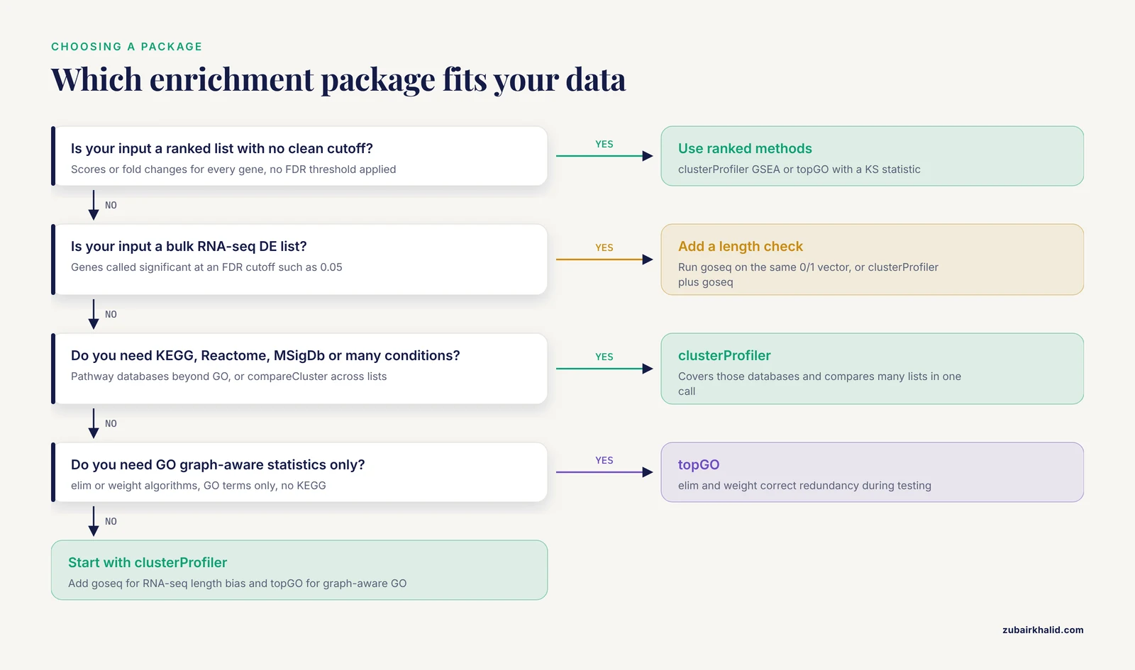
The rule of thumb: start with clusterProfiler, add goseq when your input is a bulk RNA-seq differential expression list, and reach for topGO when you want GO-graph-aware statistics or need to test a ranked score without choosing a cutoff. The rest of this article explains when those defaults flip, with working code for all three.
All three packages are free, open source, and distributed through Bioconductor, the standard repository for R bioinformatics software. Everything below doubles as a compact Bioconductor tutorial: installation commands, minimal working examples, and worked scenarios modeled on published studies.
The Short Answer
- Most projects: clusterProfiler. It covers GO, KEGG, MSigDb, and custom gene sets, runs both ORA and GSEA, compares many conditions in one call, and produces the figures reviewers expect.
- Bulk RNA-seq differential expression lists: goseq, or clusterProfiler plus a goseq sensitivity check. If long genes dominate your DE list, uncorrected ORA can manufacture enrichment.
- GO-only questions with graph-aware statistics: topGO. Its elim and weight algorithms stop broad parent terms from claiming significance that one specific child term actually drove.
- A ranked list with no clean cutoff: clusterProfiler GSEA, or topGO with a Kolmogorov-Smirnov statistic. Both avoid thresholding entirely.
- A non-model species: clusterProfiler or goseq with a custom gene set mapping built from your own annotation.
What Enrichment Analysis Actually Tests
Functional enrichment analysis is a cornerstone of interpreting high-throughput transcriptomics and proteomics data, because raw identifier lists say little until they are placed in the context of pathways, processes, and mechanisms [1]. Two related tests do most of that work.
Over-representation analysis (ORA) starts with a list of interesting genes, typically differentially expressed genes (DEGs) declared significant at a false discovery rate (FDR) below a threshold such as 0.05, and a background universe, the set of genes that could have appeared on that list. The tool counts how many genes from each annotation category, a Gene Ontology (GO) term or a Kyoto Encyclopedia of Genes and Genomes (KEGG) pathway, land in the interesting list, and compares that count with the hypergeometric expectation under random sampling from the universe. Each category receives a p-value, adjusted across all categories with a method such as Benjamini-Hochberg FDR.
Gene set enrichment analysis (GSEA) takes a different input. You rank every gene in the experiment, for example by signed statistic or log2 fold change, without any cutoff. The method walks down the ranked list and computes an enrichment score for each gene set based on where its members fall in the ranking. A set whose genes cluster at the top or bottom of the list scores high, and significance comes from permutation-based estimation. GSEA asks whether a set is coordinately shifted, while ORA asks whether a set is overrepresented among a thresholded list.
Every one of these packages runs the same five-step pipeline, and the differences live inside the steps:
- Define the interesting genes, or a ranking of all genes.
- Define the universe.
- Map your identifiers to categories.
- Test each category and adjust for multiple testing.
- Reduce redundancy and interpret the surviving terms.
clusterProfiler, goseq, and topGO differ in which biases they correct at steps 1 through 4, which databases they reach at step 3, and what they hand you at step 5.
clusterProfiler vs goseq vs topGO at a Glance
| Criterion | clusterProfiler | goseq | topGO |
|---|---|---|---|
| Core question | Are my genes overrepresented in gene sets, and do sets track a ranked list | Are my RNA-seq DE genes overrepresented after correcting gene length bias | Are GO terms significant after accounting for the GO graph |
| Methods | Hypergeometric ORA, GSEA with efficient fgsea-based estimation | Wallenius noncentral hypergeometric, sampling, or plain hypergeometric | classic, elim, weight, weight01 algorithms with Fisher or Kolmogorov-Smirnov statistics |
| Databases | GO, KEGG, MSigDb, Disease Ontology, Reactome (via ReactomePA), WikiPathways, custom sets | GO and KEGG for supported genomes, custom categories via gene2cat | GO only |
| Input | Character vector of IDs plus universe, or a ranked numeric vector | Named 0/1 vector plus gene lengths | Named 0/1 vector or a named score vector |
| Length bias correction | No | Yes, the core feature | No |
| GO graph handling | simplify() merges redundant terms after testing | None built in | elim and weight correct during testing |
| GSEA support | Yes | No | Score-based KS-style tests only |
| Multi-group comparison | compareCluster() in a single call | One list at a time | One list at a time |
| Visualization | dotplot, barplot, cnetplot, emapplot, ridgeplot, Cytoscape export | Minimal, mainly a diagnostic fit plot | Colored GO DAG via showSigOfNodes() |
| Custom gene sets | enricher() and GSEA() with TERM2GENE tables or GMT files | gene2cat mapping | Possible but awkward, the package is GO-centric |
| Maintenance | Very active, frequent Bioconductor releases | Stable, infrequent updates | Stable, slow-moving |
| Best fit | Most enrichment projects, pathway databases, publication figures | Bulk RNA-seq DE lists | GO-only, graph-aware, or cutoff-free testing |
The table compresses real trade-offs, so the sections below take each package on its own terms before returning to the criteria that decide actual projects.
clusterProfiler: The Flexible Default
What It Is and When to Use clusterProfiler
clusterProfiler, developed and maintained by the Yu Lab on Bioconductor, is the most widely used enrichment package in R. A current protocols workflow describes it as widely used for its robust statistical methods and versatile visualization options, spanning bar plots, dot plots, and enrichment maps, and uses it for both ORA and GSEA [1].
Use clusterProfiler when any of these apply:
- You need databases beyond GO, such as KEGG, MSigDb, Disease Ontology, Reactome through the companion ReactomePA package, or WikiPathways.
- You want ORA and GSEA in one package with one result class.
- You have several conditions, clusters, or time points to compare side by side.
- You need publication-quality figures and network exports.
- You work with custom gene sets, for example from the msigdbr package or your own GMT files (Gene Matrix Transposed, a simple two-column file format that pairs each gene set with its member genes).
A Minimal ORA Workflow
Install once from Bioconductor:
install.packages("BiocManager")
BiocManager::install(c("clusterProfiler", "goseq", "topGO"))
A typical over-representation run for human data looks like this:
library(clusterProfiler)
library(org.Hs.eg.db)

# de_symbols is a character vector of gene symbols from your DE table
de_map   <- bitr(de_symbols, fromType = "SYMBOL", toType = "ENTREZID",
                 OrgDb = org.Hs.eg.db)
de_entrez <- unique(de_map$ENTREZID)

ego <- enrichGO(
  gene          = de_entrez,
  universe      = expressed_entrez,   # genes actually detected in your experiment
  OrgDb         = org.Hs.eg.db,
  keyType       = "ENTREZID",
  ont           = "BP",
  pAdjustMethod = "BH",
  qvalueCutoff  = 0.05
)

ekk <- enrichKEGG(
  gene     = de_entrez,
  universe = expressed_entrez,
  organism = "hsa"
)
Three details in that block carry most of the practical weight. First, org.Hs.eg.db is the human Bioconductor annotation package, one of a family of org.Xx.eg.db packages for model organisms, and it supplies the GO mappings. Second, bitr() converts between identifier types, here from gene symbols to Entrez IDs, the numeric gene identifiers maintained by NCBI, because KEGG enrichment expects Entrez-style IDs and an organism code such as hsa for human. Third, the universe argument matters enormously. If you leave it out, clusterProfiler uses every gene in the annotation database as the background, which usually overstates significance because it includes genes your assay could never detect. Pass the genes you actually measured.
GSEA on Ranked Lists
For GSEA you supply a named numeric vector sorted in decreasing order, where the names are gene IDs and the values are ranking statistics such as signed log2 fold changes:
ranked <- sort(lfc, decreasing = TRUE)   # named by Entrez ID
gse <- gseGO(geneList = ranked, OrgDb = org.Hs.eg.db, ont = "BP")
clusterProfiler's GSEA functions use the estimation approach from the fgsea package, which evaluates enrichment probabilities efficiently without brute-force permutation, so genome-scale ranked lists run in seconds to minutes. The same ranked-list interface works for KEGG through gseKEGG() and for arbitrary gene sets through the generic GSEA() function with a TERM2GENE table.
Comparing Many Conditions at Once
compareCluster() runs the same enrichment across several gene lists in one call and returns one object you can plot as a single figure:
clusters <- list(early = early_entrez, late = late_entrez)
cc <- compareCluster(geneCluster = clusters, fun = "enrichGO",
                     OrgDb = org.Hs.eg.db, ont = "BP")
dotplot(cc, showCategory = 10)
This single feature settles the clusterProfiler or goseq question for time courses, single-cell clusters, and multi-condition experiments, because goseq and topGO process one list at a time.
Visualization, Redundancy Reduction, and Network Export
The enrichplot ecosystem that ships alongside clusterProfiler turns result objects into dot plots, bar plots, category-gene network plots (cnetplot), enrichment map plots (emapplot), ridge plots of fold change distributions per term, and heat plots. Because GO terms overlap heavily, run simplify() on GO results, which uses semantic similarity between terms to merge near-duplicate categories into one representative.
A recent protocols workflow extends this output into network space. It performs ORA and GSEA with clusterProfiler, calculates term similarity between enriched terms, and exports the resulting networks to Cytoscape with its cyemapplot function, demonstrating three complementary styles: basic networks that reveal functional modules, pie chart networks that quantify pathway coverage so you can prioritize complete versus partial perturbations, and networks that integrate expression directionality [1]. That pipeline is a good template when your enriched term list runs into the hundreds and static dot plots stop being readable.
Custom Gene Sets and Non-Model Organisms
enricher() accepts any TERM2GENE data frame, so MSigDb sets from msigdbr, gene sets from a GMT file read with fgsea's read.gmt(), or categories you built yourself all work through the same interface. The GSEA() function takes the same tables for ranked analyses. This is also the door for non-model organisms, covered in the worked scenarios below.
goseq: Correcting Gene Length Bias in RNA-seq
Where Length Bias Comes From
In bulk RNA-seq, the number of reads mapping to a gene scales with both its expression level and its length. A longer transcript captures more fragments at equal expression, so long genes tend to accumulate higher counts, more precise variance estimates, and more statistical power to be called differentially expressed. If a GO term happens to contain mostly long genes, its members pile up in the DE list for statistical rather than biological reasons, and uncorrected ORA reports that term as enriched. This selection bias is the documented motivation for goseq, which was built specifically for gene set testing on RNA-seq results.
The bias is not hypothetical. It appears whenever the genes called significant have a systematically different length distribution from the genes that were tested, which is common in standard bulk RNA-seq differential expression tables.
The goseq Workflow
goseq runs in two steps. First, nullp() fits the probability weighting function (PWF), a curve describing the probability that a gene is differentially expressed as a function of its length. Second, goseq() tests each category under a Wallenius noncentral hypergeometric approximation, a sampling model that reweights the null so that length-driven selection is accounted for:
library(goseq)

# de_genes: named numeric vector, 1 for DE genes, 0 otherwise,
# names are gene IDs matching the genome tables
pwf <- nullp(de_genes, genome = "hg38", id = "ensGene")
go_res <- goseq(pwf, genome = "hg38", id = "ensGene")
head(go_res[go_res$over_represented_pvalue < 0.05, ])
The result data frame reports over_represented_pvalue, under_represented_pvalue, the number of DE genes in the category, and the category size, with the usual multiple-testing adjustment. Several options extend the basic recipe:
- method = "Sampling" performs an exact Monte Carlo test instead of the Wallenius approximation. It is slower and usually changes little.
- method = "Hypergeometric" reproduces the uncorrected result, which is useful as an internal control to see how much the correction matters for your data.
- The bias.data argument lets you model a covariate other than length, for example GC content, if that is what drives detection in your assay.
- A custom gene2cat mapping replaces the built-in genome tables, which makes goseq work for any species and any category set.
- KEGG categories can be requested alongside GO for supported genomes.
supportedGenomes() lists the genome assemblies and identifier types goseq knows out of the box.
When the Correction Matters, and When It Does Not
- Read the diagnostic plot nullp() produces. A roughly flat fitted curve means length and DE status are unrelated in your data, and plain hypergeometric testing is defensible.
- The correction targets ORA on DE lists from bulk RNA-seq. It does not apply to proteomics, where detection depends on peptide properties rather than transcript length.
- goseq performs ORA only. There is no GSEA mode, and plotting is limited to the diagnostic fit, so most analysts pair it with clusterProfiler for figures and for pathway databases beyond GO and KEGG.
- Because the universe is defined by the 0/1 vector you pass in, goseq gives you no way to accidentally use the whole annotation as background, which quietly removes the most common ORA error.
topGO: Tests That Respect the GO Graph
Why Plain ORA Misreads the GO Hierarchy
The Gene Ontology is a directed acyclic graph (DAG), a hierarchy in which genes annotated to a specific term are implicitly annotated to all of its parent terms. That structure creates a redundancy problem for plain ORA. When one specific term is genuinely significant, every broad ancestor inherits its genes and often reaches significance too, so a results table full of overlapping terms can reflect a single biological signal counted many times. Standard per-term Fisher tests ignore this structure entirely.
The elim and Weight Algorithms
topGO attacks the problem during testing rather than after. Four algorithms are available:
- classic is the plain per-term test, equivalent to any ORA tool.
- elim traverses the GO graph from the most specific terms upward. Once a term is called significant, its genes are removed from the parent's contingency table, so a parent only reaches significance on evidence not already explained by its children.
- weight keeps all genes but downweights a term's evidence when neighboring terms in the graph already account for it.
- weight01 combines weight and elim behavior and is a common practical choice.
The nodeSize argument drops terms with very few annotated genes, for example nodeSize = 10, which reduces noise from tiny categories.
library(topGO)

topDiffGenes <- function(allScore) {
  return(allScore < 0.01)   # allScore holds per-gene p-values
}

go_data <- new("topGOdata",
               ontology = "BP",
               allGenes = gene_pvalues,        # named numeric vector
               geneSelectionFun = topDiffGenes,
               annot = annFUN.gene2GO,
               gene2GO = geneid2go,
               nodeSize = 10)

res_elim <- runTest(go_data, algorithm = "elim", statistic = "fisher")
GenTable(go_data, elimFisher = res_elim, topNodes = 20)
Here geneid2go is a list you build from your annotation, mapping each gene to its GO terms, and annFUN.gene2GO consumes it. Model organism org.Xx.eg.db packages plug in through other annot functions if you prefer.
Testing Ranked Scores Without a Cutoff
The same topGOdata object accepts all genes with continuous scores and supports Kolmogorov-Smirnov style statistics:
res_ks <- runTest(go_data, algorithm = "classic", statistic = "ks")This tests whether the genes of a term sit unusually far up a ranking of all genes, which sidesteps thresholding altogether. When no FDR cutoff yields a workable gene list, or when you distrust the cutoff you have, this is the cleanest GO-only alternative to GSEA.
Output and Limits
score() extracts p-values per term, GenTable() assembles a comparison table across algorithms, and showSigOfNodes() draws the GO DAG with significant terms shaded, which is often the single most informative GO figure because it shows where in the hierarchy the signal lives. The limits are equally clear. topGO covers GO only, has no KEGG support, offers no identifier conversion, and its interface and development pace are older than clusterProfiler's. Choose it for its statistics, not its ecosystem.
How to Choose: The Criteria That Decide Real Projects
Input Data and Study Design
A thresholded list with a defensible universe points toward ORA, and all three packages do ORA. A ranked list with no natural cutoff points toward GSEA in clusterProfiler or a KS statistic in topGO. Many conditions or clusters point to clusterProfiler, because compareCluster() removes the loop you would otherwise write around goseq or topGO.
Databases and Ontologies
If your question lives in KEGG, Reactome, MSigDb, or disease ontologies, clusterProfiler is the only one of the three that gets you there without manual plumbing. goseq reaches GO and KEGG for supported genomes plus anything you map yourself. topGO reaches GO and nothing else. For a non-model species, both clusterProfiler and goseq accept custom mappings, and the effort is in building the annotation rather than running the test.
Statistical Assumptions
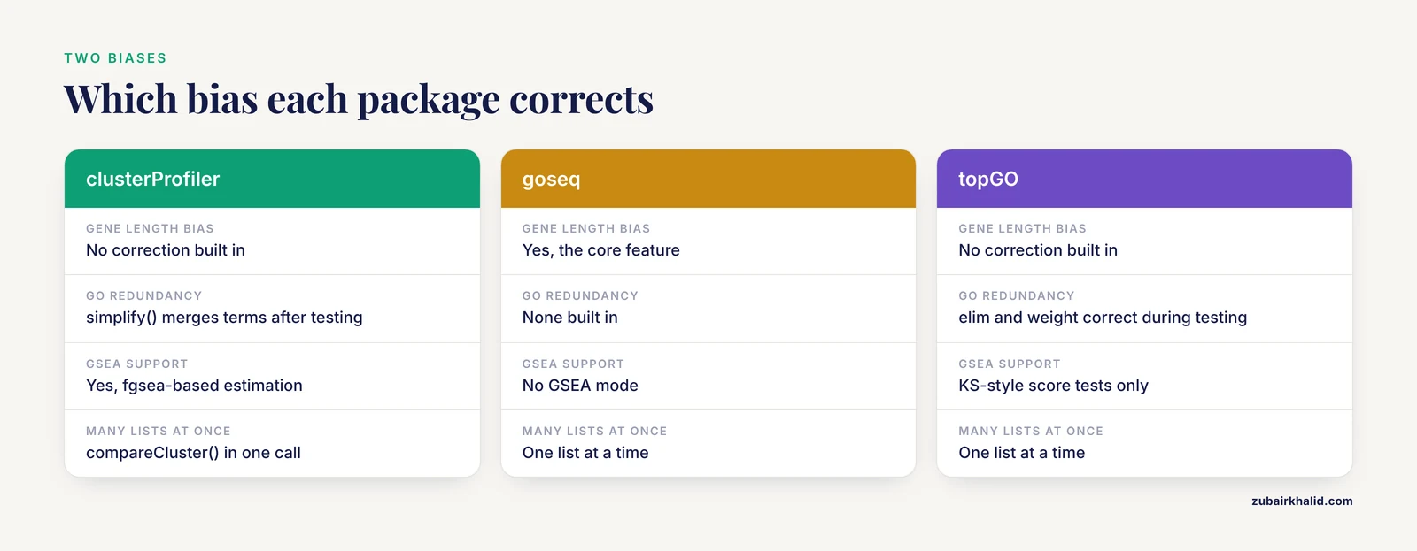
Two biases threaten enrichment results, and no single package corrects both. Gene length bias in RNA-seq DE lists is corrected by goseq. Redundancy from the GO hierarchy is handled by topGO's elim and weight algorithms during testing, or by clusterProfiler's simplify() after testing. Decide which bias threatens your specific conclusion more, or run two tools and report where they agree. Agreement between a length-corrected result and a graph-aware result is a strong signal.
Output, Maintenance, and Reproducibility
clusterProfiler has the largest documentation footprint, the most active release cycle, and the richest visualization, which matters when figures carry the paper. Whichever package you choose, keep the enrichment step scripted, record package and database versions with sessionInfo(), and fix the universe in code rather than leaving it implicit. A published computational and statistical framework for quantitative proteomics models this habit well, structuring the entire analysis as reproducible off-the-shelf R code with ORA and GSEA as explicit scripted steps and the complete script available publicly [2].
Worked Scenarios
Scenario 1: Bulk RNA-seq With DESeq2 Results
You ran DESeq2, applied log2 fold change shrinkage, and pulled DEGs at FDR below 0.05. The standard plan is enrichGO() and enrichKEGG() in clusterProfiler on Entrez-converted IDs with the expressed genes as universe, then a goseq run on the same 0/1 vector as a length bias check. Published RNA-seq workflows follow exactly this shape. A transcriptome analysis of deltamethrin resistance in Aedes aegypti populations from Metro Manila performed differential expression on RNA-seq data, then GO and KEGG analyses revealed enrichment of cytochrome P450-related terms and xenobiotic metabolism pathways, with selected genes validated by qPCR at a correlation of R = 0.89 [3]. For this kind of project the practical answer to clusterProfiler or goseq is both, with clusterProfiler carrying the figures and pathway databases and goseq confirming that the GO picture survives length correction.
Scenario 2: Quantitative Proteomics
Mass spectrometry proteomics has no transcript length bias, so goseq drops out. The universe is the set of proteins identified in your experiment, not all annotated proteins, and identifiers are often UniProt accessions or gene symbols that need conversion before KEGG queries. A published step-by-step proteomics pipeline builds exactly this flow in R, moving from preprocessing and differential abundance testing to functional enrichment with ORA and GSEA and then to interaction network construction, with complete reproducible code provided [2]. Applied examples show the payoff. A species-resolved proteomics study of breast cancer xenograft models identified 577 proteins differentially abundant between tumor and healthy mammary tissue, and functional enrichment pointed to altered lipid metabolism pathways [4]. Proteomic profiling of pancreatic alpha, beta, and delta cells isolated by laser microdissection identified cell-type-specific proteins, with beta cells showing distinct enrichment patterns [5]. A combined ultrastructure and bone proteome study reported coupling between immune and osteogenic signaling pathways [6]. For GO-centric proteomics questions, topGO's elim algorithm is a strong fit, because proteomics gene lists are small and redundant parent terms are a real nuisance at that scale.
Scenario 3: Many Conditions, Clusters, or Time Points
You have DE lists from six time points or twelve single-cell clusters and one figure to hold them. compareCluster() in clusterProfiler runs every list through the same test and returns one object that dotplot() renders as a grouped comparison. goseq and topGO would each need a hand-written loop and manual figure assembly, and neither produces a combined object. This is one of the clearest cases for when to use clusterProfiler.
Scenario 4: A Non-Model Species
No org.Xx.eg.db package exists for your organism, so you build the annotation yourself: protein evidence from BLAST or orthology tools, functional assignment from domain and orthology prediction, then gene set files in GMT format. ShEnrich, a functional annotation and enrichment platform for penaeid shrimp, did exactly this, constructing GMT libraries for KEGG and GO and implementing the enrichment with clusterProfiler, integrating 61,287 annotated proteins representing 34,169 genes, 178,595 gene-pathway associations across 442 KEGG pathways, and 138,077 proteins mapped to 12,897 GO terms across five farmed species [7]. The same custom tables feed clusterProfiler's enricher() and GSEA() directly, and feed goseq through gene2cat if you also want length correction on shrimp RNA-seq lists.
Scenario 5: Screen Hits and Ranked Lists With No Natural Cutoff
Perturbation screens and genome-wide functional assays often produce scores rather than clean hit lists. Two routes avoid arbitrary thresholds: clusterProfiler GSEA on the ranked scores, or topGO with a KS statistic on the same scores. A genome-wide functional analysis of conserved human intronic regions illustrates the payoff of set-based thinking on such data, finding that genes harboring highly conserved intronic sequences were enriched for functions in RNA processing, chromatin remodeling, and neuronal biology [8]. Whether that signal survives depends on testing all genes coherently, which is what ranked methods do.
A Note on Metabolomics
The same enrichment logic extends beyond genes, but these three packages are gene-centric and will not metabolite-map for you. A published methods chapter on metabolomics data analysis in R covers enrichment analysis using prior knowledge networks, integrated with proteomics through multi-omics factor analysis, as a framework for biomarker discovery [9]. If your study spans metabolites and transcripts, plan the metabolite enrichment with metabolite-focused resources and keep clusterProfiler, goseq, or topGO for the gene side of the integration.
Common Mistakes and Limitations
- Using the default universe. Running enrichGO() without universe= tests your DE list against every annotated gene, including hundreds your assay never observed, and inflates significance. Pass the genes detected in your experiment. goseq avoids this error structurally because the universe is whatever you pass as the 0/1 vector.
- Mixing identifier types. Feeding gene symbols where Entrez IDs are expected silently produces empty or garbage results. Convert with bitr() or your own mapping, and check how many genes the conversion dropped, because a mapping that loses a third of your list changes the test.
- Thresholding when you have a ranking. Cutting a ranked list at an arbitrary FDR and then running ORA throws away order information and can miss coordinated moderate shifts. Use GSEA or a KS statistic when the ranking is the meaningful input.
- Skipping the length bias check on RNA-seq. If long genes dominate your DE list, uncorrected GO ORA can report enrichment that is an artifact of read-depth physics. Run nullp(), look at the fitted curve, and run goseq() when the curve is steep.
- Reporting redundant GO terms. A table of twenty overlapping terms is usually one finding counted twenty times. Apply simplify() in clusterProfiler or use elim in topGO, and report the merged picture.
- Over-reading small gene lists. Enrichment on a handful of genes is fragile. A multimodal analysis of PFAS-induced hepatotoxicity found that conventional pathway enrichment recapitulated known effects on SREBF- and PPAR-driven lipid metabolism but provided limited insight for compounds with fewer DEGs, such as PFBS [10]. Treat sparse-list enrichment as weak evidence and lean on targeted or network approaches when the list is small.
- Reading enrichment as activation. ORA says nothing about direction. A term enriched among DEGs can mix up- and down-regulated genes. GSEA with signed rankings preserves direction, and visualization workflows that integrate expression directionality into network views make the distinction explicit [1].
- Ignoring multiple testing details. Report adjusted p-values or q-values, not raw ones, and be skeptical of terms supported by only two or three genes, which nodeSize in topGO or minGSSize in clusterProfiler can filter.
- Forgetting annotation drift. GO, KEGG, and org.db contents change between releases, so the same script can return different terms a year later. Record package versions, database versions, and the date of KEGG retrieval in your methods.
- Treating enrichment as mechanism. Enrichment is descriptive hypothesis generation. It ranks candidate explanations, it does not prove a pathway is causally altered, and for high-stakes conclusions the analysis plan deserves review by a statistician or experienced bioinformatician, since enrichment choices are easy to get wrong quietly.
Frequently Asked Questions
Should I use clusterProfiler or goseq for an RNA-seq gene list?
Run clusterProfiler first for breadth and figures, then run goseq on the same list as a length bias check. If the two agree, report the clusterProfiler results with a note that goseq confirmed them. If they disagree, trust goseq for GO terms and report the discrepancy.
Can I use more than one of these packages in the same project?
Yes, and it is standard practice. A common pattern is goseq for the length-corrected GO result, clusterProfiler for KEGG, MSigDb, and visualization, and topGO when a reviewer asks for graph-aware GO statistics.
Do I need Entrez gene IDs?
For KEGG enrichment in clusterProfiler, yes, the function expects Entrez-style identifiers and an organism code such as hsa. GO enrichment through an OrgDb accepts other key types, including Ensembl IDs and gene symbols. goseq needs identifiers matching its genome tables or a custom mapping, and topGO needs whatever your annotation object uses.
Can topGO run KEGG pathway enrichment?
No. topGO works with the Gene Ontology only. Use enrichKEGG() in clusterProfiler, or request KEGG categories in goseq for supported genomes.
Does goseq make sense for proteomics or single-cell RNA-seq?
For proteomics, no, because transcript length does not drive protein detection. For single-cell data, the length bias argument is weaker and the package was not designed for it, so most analysts use clusterProfiler. goseq can model other covariates through its bias.data argument, but that is a custom design decision.
Which package should I learn first in R for bioinformatics?
clusterProfiler. It covers the widest range of databases, supports both ORA and GSEA, has the most extensive documentation, and its functions appear in most published enrichment workflows, so the skills transfer directly.
Sources
- Enhancing Interpretation of Functional Enrichment Analysis Results with Advanced Network Visualizations.
- Computational and Statistical Framework for Quantitative Proteomics Analysis.
- Transcriptome Analysis of Deltamethrin Resistance Mechanisms in Aedes aegypti Populations from Metro Manila, Philippines.
- Host-Derived Proteomic Profiling of Human and Canine Mammary Tumor Xenografts Identifies Enrichment of Lipid Metabolism-Related Pathways.
- Proteomic analysis of pancreatic endocrine cells by mechanistic single-cell isolation identifies membrane pathways.
- Integrated analysis of human osteocyte lacunar ultrastructure and bone proteome profiling reveals coupling between immune and osteogenic signaling pathways.
- ShEnrich: a functional annotation database and enrichment platform for penaeid shrimp.
- A genome-wide functional analysis of conserved intronic regions reveals essential roles for speckle-associated retained introns.
- Multi-Omics Guided Pathway and Network Analysis of Clinical Metabolomics and Proteomics Data.
- Multimodal cheminformatic and network biology analysis enables deeper mechanistic understanding of PFAS-induced hepatotoxicity.