How to Annotate Variants in the Cloud
By Dr. Zubair Khalid, DVM, MS, PhD ·

By the end of this guide you will be able to take a variant call format (VCF) file, upload it to a cloud virtual machine, run Ensembl Variant Effect Predictor (VEP) against a local cache, layer on supplementary annotations from a hosted web service, attach automated clinical classification, and package the whole thing as a reproducible workflow. You will need a cloud account with billing enabled (AWS, Google Cloud, or Azure all work), basic comfort with the Linux command line, a VCF aligned to a known reference build (GRCh38 in the worked examples), and about 20 GB of scratch space for caches and indexes.
Variant annotation is the step that turns a list of genomic positions into a list of biological facts. A caller gives you chr7:140453136A>T. Annotation tells you that this changes a codon in the BRAF gene, that the resulting protein change is the well-characterized V600E substitution, that the variant appears at a particular frequency in population databases, and that clinical databases have already assigned it an interpretation. Without annotation, downstream filtering and interpretation are guesses.
What Variant Annotation Actually Does
Variant calling and variant annotation are different steps, and mixing them up causes most beginner confusion. Variant calling reads aligned sequencing data (BAM or CRAM files) and emits a VCF, a text format with a header block and one line per variant position. Variant annotation reads that VCF and attaches information per variant: which gene and transcript are affected, what the consequence is at the protein level, what frequencies the variant shows in reference populations, what disease associations exist, and what computational predictors say about its impact.
The dominant annotation engines in human genomics are Ensembl VEP and ANNOVAR. Both draw on the same underlying public resources: Ensembl and RefSeq transcript models, ClinVar for clinical interpretations, gnomAD for population allele frequencies, and aggregated prediction scores from tools such as CADD, SIFT, PolyPhen, and SpliceAI distributed through the dbNSFP database. A recent nf-core-compliant Nextflow pipeline called MuSA illustrates the current state of the art by integrating VEP with 22 curated plugins (including AlphaMissense, CADD, SpliceAI, and Enformer) alongside ANNOVAR and a preconfigured dbNSFP distribution, then consolidating results into a single ranked report [1].
One distinction matters before you start. Some cloud platforms, such as GenomeVIP, orchestrate both variant discovery and annotation, running callers like GATK, Strelka, VarScan, and BreakDancer through a web interface before annotating the results [2]. This guide assumes your calling step is already done and your input is a VCF. If you still need to call variants, the same cloud principles apply, and a published pipeline for joint calling of 2,535 human genomes on the Amazon cloud showed near-linear scalability for that stage [3].
Why Annotate in the Cloud Instead of Your Laptop
Three forces push annotation off local hardware and into cloud bioinformatics environments.
First, data gravity. Sequencing projects now generate terabytes to petabytes, and downloading data to local servers is slow and expensive. GenomeVIP was built explicitly because the "download and analyze" paradigm was breaking down under the growth of resources like TCGA, and moving analysis to where the data lives removes that bottleneck [2]. When your BAM files sit in an object store, annotating them next to that store beats copying them.
Second, scale. The All of Us Research Program built Celeste, a cloud infrastructure on Amazon Web Services that processes fluctuating workloads of up to 9,000 whole-genome samples per month. Within a single AWS Region over 12 months of production, Celeste executed roughly 200 million serverless functions and coordinated 1.8 million analysis jobs, including variant calling and clinical reporting [4]. No single lab server approaches that throughput.
Third, reproducibility. Annotation results depend on software versions, database versions, and reference transcripts. A benchmarking workflow developed for clinical diagnostic assays runs entirely in the cloud so that analytical performance assessments can be repeated identically regardless of the technician, laboratory, or underlying hardware [5]. Containerizing your annotation stack gives you the same property for research work.
Choosing a Cloud Environment for Variant Annotation
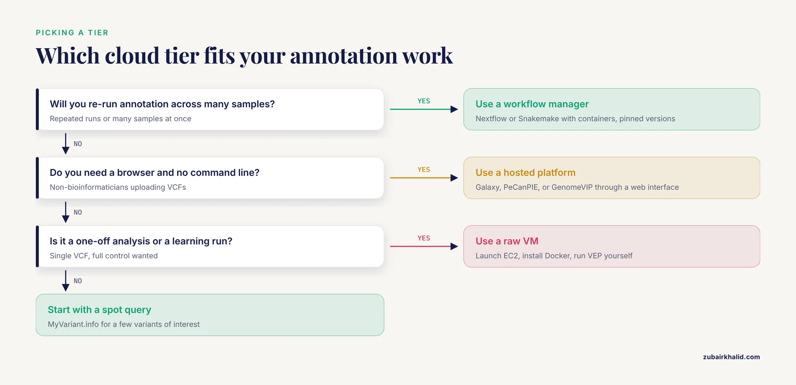
There are four practical tiers, and the right one depends on your scale and your compliance needs.
Tier 1: Raw virtual machines on AWS, Google Cloud, or Azure
You launch a virtual machine, install Docker or Conda, and run tools directly. This tier gives maximum control and is what the step-by-step walkthrough below uses. AWS genomics workloads typically combine S3 for storage, EC2 for compute, and services like AWS Batch for parallel execution. On Azure, a published pipeline runs variant calling on long-read PacBio HiFi data with Cromwell, then merges the genomic results with clinical FHIR records and performs tertiary analysis in cloud Jupyter notebooks [6]. The trade-off is that you own every configuration decision.
Tier 2: Workflow managers with containers
Nextflow and Snakemake wrap each tool in a container, track provenance, and resume interrupted runs. The CIMAC-CIDC cancer immunotherapy network rebuilt its whole-exome and RNA-seq pipelines as modular Snakemake workflows with Docker on Google Cloud Platform specifically to improve reproducibility, precision, and recall against validated truth sets [7]. MuSA, mentioned above, is an nf-core-compliant Nextflow pipeline that automates annotation from resource setup through clinical ranking [1]. If you expect to re-run annotation repeatedly or across many samples, start at this tier.
Tier 3: Hosted platforms
DNAnexus, Terra, and similar platforms provide validated pipelines with a web interface. The 2,535-genome joint calling study cited above ran on AWS through the DNAnexus platform [3]. Galaxy is an open-source alternative, and a cloud-hosted Galaxy instance was used to implement the CGtag toolkit so that researchers without command-line experience could run annotation and filtering tools through a browser [8]. GenomeVIP offers a web interface over a curated set of variant discovery and annotation tools and has been used in projects including the TCGA PanCanAtlas and the ICGC-TCGA DREAM Challenges [2].
Tier 4: Specialized web services and curation platforms
Some annotation problems are already solved as services. MyGene.info and MyVariant.info are high-performance, free web services for querying gene and variant annotation, accessed more than three million times per month, and they demonstrate a generalizable cloud model for organizing annotation data [9]. On the clinical side, PeCanPIE is a web- and cloud-based platform that accepts VCF files containing millions of variants, annotates and ranks them, and presents a decision-support interface for formal pathogenicity classification based on American College of Medical Genetics and Genomics (ACMG) guidelines [10]. For structural variants, SV-plaudit provides a cloud framework where reviewers visually assess each variant call and the system emits an annotated VCF of consensus decisions [11].
| Tier | Best for | You manage | Reproducibility mechanism |
|---|---|---|---|
| Raw VM | One-off analyses, learning | OS, tools, caches | Manual (scripts, logs) |
| Workflow manager | Repeated runs, many samples | Pipeline definition | Containers plus workflow engines [7][1] |
| Hosted platform | Regulated or collaborative settings | Little | Platform-validated pipelines [3][2][8] |
| Web service | Spot queries, small VCFs | Almost nothing | Service versioning [9] |
Step by Step: How to Annotate Variants in the Cloud
The walkthrough below annotates a germline VCF on an AWS EC2 instance. Every command translates directly to a Google Cloud VM or an Azure VM with only the storage and launch commands changed.
Step 1: Launch a compute instance
Query the latest Amazon Linux 2023 machine image through the public Systems Manager parameter, then launch a memory-optimized instance. Annotation is mostly single-machine work, so an 8-vCPU, 64 GB instance is a sensible default for a whole-exome VCF, and a larger instance for whole-genome outputs with many plugins.
# Get the current Amazon Linux 2023 AMI id
AMI_ID=$(aws ssm get-parameters \
  --names /aws/service/ami-amazon-linux-latest/al2023-ami-kernel-default-x86_64 \
  --query 'Parameters.Value' --output text)

aws ec2 run-instances \
  --image-id "$AMI_ID" \
  --instance-type r6i.2xlarge \
  --key-name my-keypair \
  --block-device-mappings '[{"DeviceName":"/dev/xvda","Ebs":{"VolumeSize":200,"VolumeType":"gp3"}}]'
Then connect:
ssh -i ~/.ssh/my-keypair.pem ec2-user@<public-ip-address>The parameters that matter here are -instance-type (choose memory over clock speed for annotation, because cache loading and plugins are memory hungry) and the root volume size (200 GB covers a GRCh38 VEP cache plus a dbNSFP distribution with room to work).
Step 2: Stage your VCF from object storage
Keep the authoritative copy of your data in object storage, not on the instance. Copy the file down, and plan to copy results back up.
aws s3 cp s3://my-project-bucket/variants/sample.vcf.gz .
aws s3 cp s3://my-project-bucket/reference/GRCh38.fa .
aws s3 cp s3://my-project-bucket/reference/GRCh38.fa.fai .
Step 3: Install Docker and validate the VCF
sudo dnf install -y docker
sudo systemctl start docker
sudo usermod -aG docker ec2-user
# log out and back in for the group change to apply
Before annotating, check that the file is a well-formed, indexed VCF. A damaged or non-block-compressed file is the single most common input failure.
# Install bcftools, samtools, and htslib utilities
sudo dnf install -y bcftools samtools

# Confirm the file opens and count variants
bcftools view -H sample.vcf.gz | wc -l
Expected output is a plain integer, for example:
4,512,877Normalize the file so that multiallelic records are split and left-aligned against the reference. Downstream tools, especially ACMG classifiers and database cross-references, assume normalized representation.
bcftools norm -f GRCh38.fa -m -both -c w sample.vcf.gz -Oz -o sample.norm.vcf.gz
tabix -p vcf sample.norm.vcf.gz
Expected output from bcftools norm:
Lines total/split/realigned/skipped: 4512877/19342/16021/0The -c w flag warns rather than exits when a REF allele does not match the reference, which surfaces build mismatches early. A nonzero skipped count means you have broken records to investigate before annotating.
Step 4: Run the first VEP pass with a local cache
VEP can annotate against an online Ensembl database or against a prebuilt local cache. On the cloud, use the cache. It is faster, it removes network dependence from the hot loop, and it pins the database version for reproducibility.
# Pull VEP from Docker Hub (check the registry for the current release tag)
docker pull ensemblorg/ensembl-vep:release_112.0

# Download the GRCh38 cache once, into a persistent directory
docker run -v "$PWD":/data ensemblorg/ensembl-vep:release_112.0 \
  --install --auto ap --species homo_sapiens --assembly GRCh38 \
  --dir_cache /data/vep_cache
Then run the annotation:
docker run -v "$PWD":/data ensemblorg/ensembl-vep:release_112.0 \
  --input_file /data/sample.norm.vcf.gz \
  --output_file /data/sample.vep.vcf.gz \
  --vcf --compress_output bgzip \
  --cache --offline --assembly GRCh38 \
  --dir_cache /data/vep_cache \
  --fasta /data/GRCh38.fa \
  --hgvs --hgvsg --symbol --biotype --numbers \
  --canonical --mane --protein --check_existing \
  --force_overwrite
Each parameter earns its place:
| Option | What it does | Why it matters |
|---|---|---|
-cache, offline | Uses the local cache with no database connection | Fast, deterministic, survives network issues |
-assembly GRCh38 | Selects the genome build | Must match the build your caller used, or every position is wrong |
-dir_cache | Cache location | Keep it in a persistent volume so repeated runs skip the download |
-fasta | Reference sequence for HGVS and sequence checks | Required for HGVS notation on a cache-only run |
-hgvs, hgvsg | Adds transcript-level and genomic HGVS names | The standard reporting vocabulary for variants |
-canonical, mane | Flags representative transcripts, including MANE Select | Reduces ambiguity in clinical reporting |
-check_existing | Matches variants against Ensembl variation databases | Attaches existing rsIDs |
-vcf, compress_output bgzip | Emits block-compressed annotated VCF | Keeps the file indexable for downstream tools |
-pick (optional) | Reports one consequence per variant | Shrinks whole-genome outputs dramatically when you do not need all transcripts |
Step 5: Inspect the output
Extract the annotation table to check results quickly:
docker run -v "$PWD":/data ensemblorg/ensembl-vep:release_112.0 \
  --input_file /data/sample.vep.vcf.gz --tab --fields \
  "Uploaded_variation,Location,Allele,Gene,SYMBOL,Consequence,EXON,HGVSc,HGVSp,EXISTING_VARIATION,MANE" \
  --no_stats -o /data/sample.vep.tsv
head -3 sample.vep.tsv
Expected output looks like this (values illustrative, format exact):
## Uploaded_variation  Location        Allele  Gene       SYMBOL  Consequence  EXON    HGVSc                     HGVSp              EXISTING_VARIATION  MANE
1:762273G>A           1:762273        A       ENSG00...  OR4F5   missense_variant,splice...   2/3     ENST00000342066.4:c.79G>A ENSP00...p.R27H    rs12123...          N
1:877754C>T           1:877754        T       ENSG00...  SAMD11  synonymous_variant           9/10    ENST00000342066.4:c.912C>T ENSP00...p.=       rs140...            N
Each row is one variant-transcript pair. The Consequence column carries Sequence Ontology terms such as missense_variant, synonymous_variant, frameshift_variant, and splice_acceptor_variant. If your output shows consequences but the gene symbols look scrambled, go directly to the build-mismatch check in the errors section.
Step 6: Layer on prediction scores and richer annotation
The base VEP run gives consequence and identity. Clinical prioritization needs deleteriousness and conservation scores. The cleanest route is the dbNSFP plugin, which joins dozens of precomputed scores onto each variant, or individual plugins for specific scores. MuSA's design, which runs VEP with 22 curated plugins including CADD and SpliceAI in parallel containerized branches, reflects how production pipelines structure this step [1].
# Example: CADD and SpliceAI plugins (each plugin requires its own
# data file downloaded from the VEP plugins documentation, plus --dir_plugins)
docker run -v "$PWD":/data ensemblorg/ensembl-vep:release_112.0 \
  --input_file /data/sample.norm.vcf.gz \
  --output_file /data/sample.vep.scores.vcf.gz \
  --vcf --compress_output bgzip \
  --cache --offline --assembly GRCh38 \
  --dir_cache /data/vep_cache \
  --fasta /data/GRCh38.fa \
  --hgvs --symbol --mane --canonical \
  --dir_plugins /data/vep_plugins \
  --plugin CADD --plugin SpliceAI \
  --force_overwrite
For a small number of variants of particular interest, you can supplement with a hosted query. MyVariant.info serves annotations aggregated from many resources through a simple REST interface and is free to the research community [9]. Query the well-known BRAF V600E variant:
curl -s "https://myvariant.info/v1/variant/chr7:140453136A>T?fields=clinvar,gnomad_exome,cadd,hgvs"Expected output (trimmed):
{
  "_id": "chr7:140453136A>T",
  "clinvar": {"rcv": "...", "clinical_significance": "Pathogenic", ...},
  "cadd": {"predel": "DELETERIOUS", ...},
  "gnomad_exome": {"af": {"af": 0.00001, ...}},
  "hgvs": {"genomic": ["NC_000007.14:g.140453136A>T"], ...}
}
This pattern is useful for interactive curation, not for batch work on millions of variants. Batch = cache, spot query = web service.
Step 7: Attach clinical classification
Annotation and interpretation are separate acts. Automated classifiers map annotated variants onto ACMG and AMP evidence criteria. MuSA integrates automated ACMG/AMP classification through GeneBe and InterVar as part of its pipeline [1]. PeCanPIE takes a platform approach, annotating uploaded VCFs, ranking variants by putative pathogenicity, and presenting a decision-support interface built on published ACMG guidelines, and it has been used to classify variants in cancer predisposition genes across more than 4,000 pediatric cancer patients [10]. If your use case is research-grade pharmacogenomics rather than diagnosis, a purpose-built cloud pipeline called Pgxtools identifies actionable variants in 13 pharmacogenes and generates reports annotated with clinical practice guideline interpretations [12].
Treat automated classifications as a first pass. The ACMG framework assigns evidence codes that ultimately require human judgment, and cloud tooling makes that judgment faster, not unnecessary.
Step 8: Validate against truth sets
Run a benchmark before you trust an annotation stack, especially if results inform clinical work. The Genome in a Bottle (GIAB) consortium publishes reference samples with benchmark variant calls for precisely this purpose. A scalable cloud-based benchmarking workflow chains standard comparison tools such as hap.py and vcfeval, evaluates performance across genomic regions and variant types, and removes dependence on the local hardware and library stack so assessments repeat reliably [5]. The practical sequence: run your pipeline on a GIAB sample, compare your output to the benchmark calls with one of those tools, and record sensitivity, precision, and regional performance as baseline metrics for your configuration.
Step 9: Package the workflow and control costs
Convert your commands into a Nextflow or Snakemake pipeline with pinned container versions. The CIDC team moved to Snakemake and Docker on GCP for exactly this reason, and benchmarked the rebuilt pipelines against truth sets before release [7]. Add these cost and reproducibility habits:
# Keep the authoritative outputs in object storage, then stop the instance
aws s3 cp sample.vep.vcf.gz s3://my-project-bucket/annotated/
aws s3 cp sample.vep.tsv  s3://my-project-bucket/annotated/

# When finished
aws ec2 stop-instances --instance-ids i-0123456789abcdef0
For population-scale workloads, Celeste's architecture shows the pattern that holds up at scale: serverless functions for orchestration, container orchestration for the heavy jobs, and everything within a single cloud region to keep data transfer coherent [4]. You do not need 200 million function invocations to benefit from the same shape of design.
Common Errors and How to Fix Them
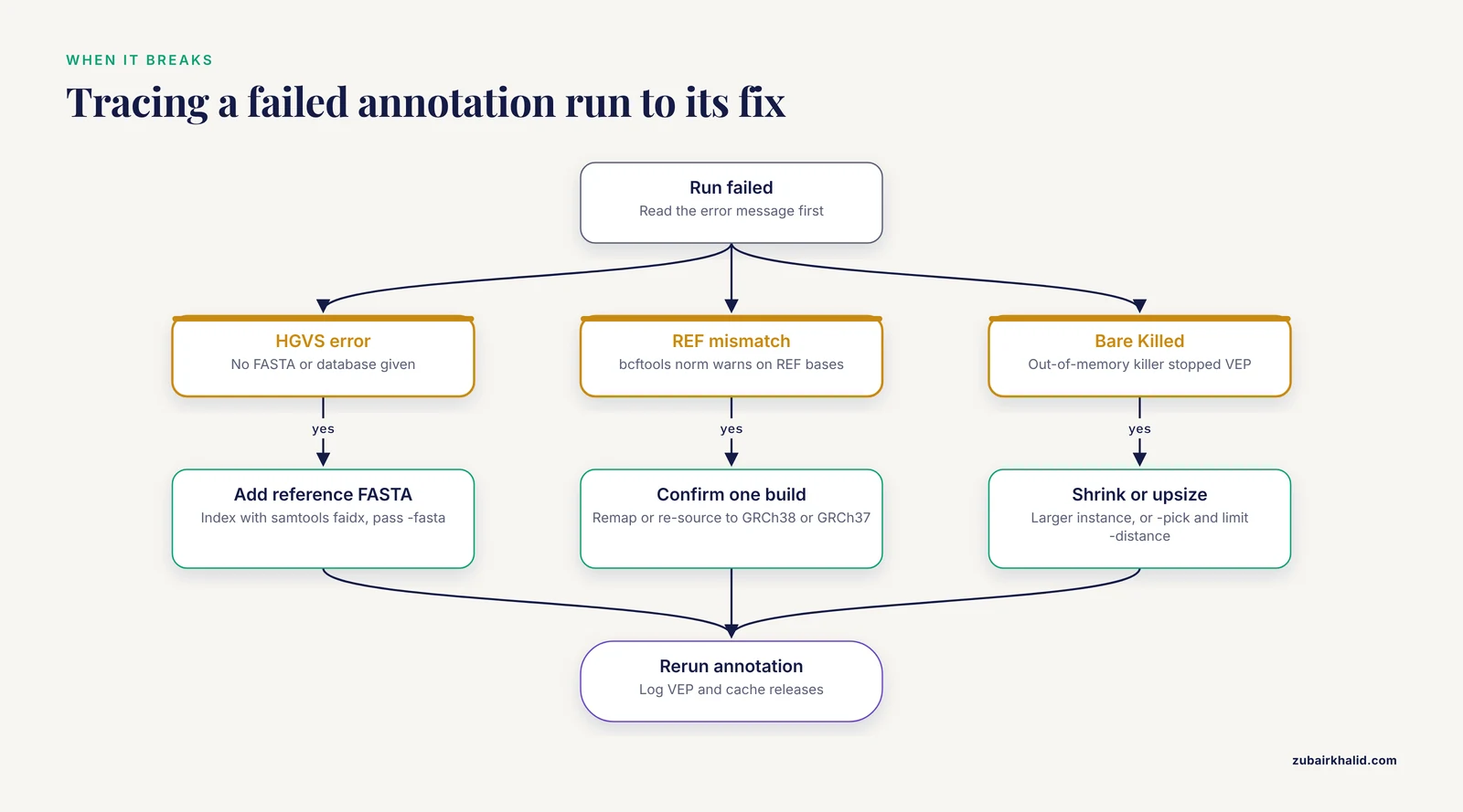
These are the failures you will actually hit, with their typical messages and fixes.
"ERROR: Cannot generate HGVS identifiers without either a FASTA file or a database." You requested -hgvs on an offline cache run without supplying -fasta. Download the reference FASTA for your build, index it with samtools faidx, and add -fasta /data/GRCh38.fa.
"Reference allele mismatch" from bcftools norm. Your VCF's REF bases disagree with your reference FASTA. Almost always this means your VCF is GRCh37 (hg19) while your FASTA is GRCh38, or vice versa. Stop and confirm the build of every input. Do not proceed with -c w and ignore thousands of warnings. Remap or re-source the file to a single consistent build.
"[E::hts_open_format] Failed to open file" or a missing-index complaint from tabix. The VCF is not block-compressed with bgzip, or the .tbi index is absent. Run bgzip -c sample.vcf > sample.vcf.gz then tabix -p vcf sample.vcf.gz. Tools that accept plain VCFs usually still run faster on the indexed form.
"Cannot connect to the Docker daemon at unix:///var/run/docker.sock." The Docker service is not running, or your user lacks permission. Run sudo systemctl start docker, and either add yourself to the docker group (sudo usermod -aG docker $USER, then log out and back in) or prefix commands with sudo.
A cache version mismatch error naming different VEP and cache versions. VEP cache releases are tied to specific VEP releases. Re-pull the matching Docker tag, or reinstall the cache for your VEP version with the -install command shown in Step 4. Recording the VEP release and cache release in your workflow log prevents recurrence.
The process dies with a bare "Killed." The Linux out-of-memory killer terminated VEP, typically during cache loading or plugin table joins. Move to a larger instance type, or reduce annotation scope with -pick and by limiting -distance, the window for upstream and downstream consequence assignment.
Gene symbols or positions that look plausible but fail every cross-check. This is the signature of a reference build mismatch that slipped past normalizing, or of mixing transcript sets between annotation runs. The fix is disciplined build tracking, covered below.
How to Check That the Annotation Is Right
Verification has four layers, cheap to expensive.
First, spot-check known variants. BRAF V600E should annotate as a missense variant in BRAF with pathogenic status in ClinVar, and a -check_existing run should attach its rsID. If your pipeline mislabels a variant this famous, everything downstream is suspect.
Second, cross-check against an independent service. Query a sample of variants through MyVariant.info and confirm that consequence, gene, and population frequency fields agree with your batch output [9]. Agreement between a cache-based tool and a service-based source is strong evidence the build and transcript selection are consistent.
Third, benchmark formally. Run GIAB reference samples through your full annotation configuration and compare with hap.py or vcfeval, as the clinical benchmarking workflow demonstrates [5]. This is the standard for anything diagnostic-adjacent.
Fourth, for structural variant calls where automated annotation is weakest, add human review. SV-plaudit was built because SV evidence images benefit from expert eyes. It generates visualization images per variant, distributes them through a cloud web application for scoring, and emits an annotated VCF of the consensus assessments. In its proof of principle, nine researchers each evaluated 1,350 structural variants in one hour [11]. If your pipeline calls SVs, budget curation time proportionally.
Tips for Faster, Cheaper, Cleaner Cloud Annotation
Keep the cache warm and shared. Put the VEP cache and plugin data files in a persistent volume or a shared filesystem that instances mount, rather than re-downloading per run. At population scale this is the difference between trivial and painful overhead.
Match instance shape to workload. Annotation parallelizes poorly within a single variant record but parallelizes perfectly across chromosomal chunks. Split your VCF by chromosome, run parallel jobs, and concatenate. Given the near-linear scalability demonstrated for cloud variant calling at cohort scale, the same economics apply to annotation [3].
Pin everything. Record the VEP release, cache release, plugin versions, dbNSFP version, container digests, and reference FASTA checksums in your workflow log. The entire value of cloud bioinformatics for annotation collapses if the databases drift between runs, which is why production pipelines lean on containers and workflow engines [7].
Use spot or preemptible instances for batch annotation, with checkpointing from a workflow manager so preemption costs minutes rather than hours.
Reduce output before you reduce compute. Whole-genome VCFs annotated against all transcripts generate enormous files. If your downstream analysis reads one consequence per variant, -pick shrinks runtime and storage together.
Use services where they exist. Free, maintained services such as MyVariant.info handle aggregated annotation queries at millions of requests per month, and reimplementing that aggregation locally buys you nothing [9].
Common Mistakes and Limitations
Reference build confusion. Mixing GRCh37 and GRCh38 coordinates across inputs, caches, and FASTA files silently produces wrong annotations that still look plausible. Confirm the build at every hand-off, and state it in every output filename and log.
Skipping normalization. Unsplit multiallelics and unnormalized indels fail to match database keys, so variants lose their ClinVar records and frequency data for no biological reason. Always run bcftools norm upstream.
Treating prediction scores as verdicts. CADD, SIFT, SpliceAI, and AlphaMissense scores are evidence, not diagnoses. The ACMG classification frameworks embedded in tools like InterVar, GeneBe, and PeCanPIE exist because pathogenicity requires combining multiple evidence types, and human review remains part of the standard [10][1].
Mixing cases with public controls whose pipelines differ. If you annotate your cases with one pipeline and pull frequencies from external datasets processed differently, association tests can inflate false positives. A systematic analysis using gnomAD v2.1 and in-house datasets found that inflated test statistics decreased substantially when the same variant caller and filtering pipelines were applied to cases and controls, while differences in library prep kits and sequencers did not drive inflation, and joint versus separate calling did not either [13]. The lesson for annotation is that pipeline provenance is a scientific variable, not a convenience.
Assuming reproducibility without testing it. Benchmarking tools such as hap.py and vcfeval depend on hardware and software libraries, which is precisely why the clinical benchmarking workflow was containerized and run in the cloud [5]. If you have not benchmarked your annotation stack, you do not know its performance characteristics.
Uploading identifiable patient data to services that were not designed for it. Some researchers moved toward standalone, in-situ pipelines explicitly because reliance on cloud services with nontransparent internal processing raised safety concerns for patient data in settings with limited connectivity [14]. Where you do use the cloud for clinical data, choose platforms built for it, such as pipelines that handle FHIR clinical records and genomic data together under one secure design [6], and make sure your data-use agreement and institutional policy cover the destination.
Paying for idle compute. The most common self-inflicted cloud cost is an instance left running over the weekend after a job finished. Put stop-and-snapshot logic in your workflow and check the console before signing off.
Expecting LLMs to replace annotation pipelines. Retrieval-augmented generation over 190 million curated variant annotations substantially improved GPT-4o's ability to answer variant queries, and outperformed fine-tuning on accuracy and cost, but annotation fields outside the integrated datasets remained imperfectly answered [15]. Use language models as an interface and reasoning layer over verified annotations, never as the annotation source itself.
Next Steps
Once single-sample annotation runs cleanly in the cloud, extend along three axes. Add samples by converting your commands into a Nextflow or Snakemake pipeline with containers, following the pattern of nf-core-compliant annotation pipelines [1]. Add depth by enabling the plugins and clinical classifiers that match your disease domain, whether that is cancer predisposition screening through platforms like PeCanPIE [10] or pharmacogenomics through dedicated pipelines [12]. Add rigor by adopting benchmarking against GIAB truth sets as a standing regression test, so every change to your annotation stack is measured against known performance [5].
Frequently Asked Questions
What are cloud variant annotation tools?
They are software systems, hosted on cloud infrastructure, that attach biological and clinical information to genomic variants listed in a VCF file. They range from command-line engines like VEP running on virtual machines, to workflow pipelines on Nextflow and Snakemake, to hosted web platforms and services such as Galaxy instances, MyVariant.info, and PeCanPIE.
How do I annotate variants in the cloud step by step?
Launch a cloud virtual machine, stage your VCF from object storage, normalize it with bcftools, run VEP in a container against a local cache for your reference build, add prediction plugins, apply ACMG-based classification if needed, validate against GIAB truth sets, and package the commands as a containerized workflow. The full walkthrough with commands is in the step-by-step section above.
How much does cloud variant annotation cost?
Published benchmarks exist for the calling stage rather than annotation alone. Joint variant calling on 2,535 human genomes ran in about five days at a compute cost of $7.33 per sample, roughly $18,590 total for completed jobs, using parallel execution on the Amazon cloud [3]. Annotation is cheaper than calling per sample, and the same parallelization economics apply.
Do I need command-line experience to annotate variants in the cloud?
No, if you choose the right platform. Cloud-hosted Galaxy instances expose annotation tools through a point-and-click web interface [8], PeCanPIE was designed so non-bioinformaticians can upload and classify variants through a browser [10], and notebook-based pipelines have been built specifically to remove the command-line barrier for researchers.
Which cloud provider is best for genomics work?
All three major providers host production genomics. AWS runs population-scale workloads like the All of Us Celeste infrastructure [4], Google Cloud hosts the Snakemake-based CIMAC-CIDC clinical research pipelines [7], and Azure hosts Cromwell-based long-read pipelines integrated with FHIR health records [6]. Choose based on where your data already lives, your institution's agreements, and your workflow manager of choice, not on a general ranking.
How do I keep patient data safe when annotating variants in the cloud?
Use platforms and pipelines designed for clinical data, keep data within a single cloud region, and confirm your institutional and contractual requirements before uploading. Security-conscious design is an explicit motivation in published clinical pipelines, including one that parses FHIR clinical records and long-read genomic data in a single secure pipeline [6], and it is a stated reason some groups prefer standalone in-situ pipelines over opaque external services [14].
Can AI language models help with variant annotation?
Yes, as an access layer rather than an annotation engine. One study integrated 190 million curated variant annotations into GPT-4o through retrieval-augmented generation, which outperformed fine-tuning on data volume, accuracy, and cost-effectiveness, though accuracy across all annotation fields remained imperfect [15]. Verify any model-generated interpretation against the underlying annotation sources.
How do I know my cloud annotations are correct?
Spot-check variants with known interpretations, cross-check a sample against an independent service like MyVariant.info, and run formal benchmarks with GIAB reference samples using comparison tools such as hap.py and vcfeval [5]. For structural variants, add structured human review through frameworks like SV-plaudit, where multiple reviewers score each call and the consensus is written back into an annotated VCF [11].
Sources
- MuSA: a Nextflow pipeline for deep, reproducible annotation and clinical ranking of genomic variants.
- GenomeVIP: a cloud platform for genomic variant discovery and interpretation.
- Inexpensive and Highly Reproducible Cloud-Based Variant Calling of 2,535 Human Genomes.
- Celeste: A cloud-based genomics infrastructure with variant-calling pipeline suited for population-scale sequencing projects.
- Benchmarking workflows to assess performance and suitability of germline variant calling pipelines in clinical diagnostic assays.
- A cloud-based pipeline for analysis of FHIR and long-read data.
- Modular and cloud-based bioinformatics pipelines for high-confidence biomarker detection in cancer immunotherapy clinical trials.
- CGtag: complete genomics toolkit and annotation in a cloud-based Galaxy.
- High-performance web services for querying gene and variant annotation.
- Pediatric Cancer Variant Pathogenicity Information Exchange (PeCanPIE): a cloud-based platform for curating and classifying germline variants.
- SV-plaudit: A cloud-based framework for manually curating thousands of structural variants.
- A New Cloud-Native Tool for Pharmacogenetic Analysis.
- Inflated expectations: Rare-variant association analysis using public controls.
- OVAS: an open-source variant analysis suite with inheritance modelling.
- Boosting GPT models for genomics analysis: generating trusted genetic variant annotations and interpretations through RAG and Fine-tuning.