How to Chunk-Process Large Genomic Files in R: Step-by-Step
By Dr. Zubair Khalid, DVM, MS, PhD ·

By the end of this guide you will be able to filter a multi-gigabyte GWAS summary statistics file, stream variants out of a compressed VCF, process sequencing reads from a BAM file in blocks, and compute per-SNP statistics from a PLINK genotype matrix, all without loading any file fully into RAM. You will also know how to size chunks against a memory budget, parallelize the work across cores, write results incrementally, and verify that a chunked run reproduces what a full load would have produced.
Chunked processing of genomic data in R is the difference between a script that dies at 90 percent of a file and one that finishes overnight on a laptop. R for bioinformatics means base R plus Bioconductor, and both were designed around interactive statistics on modest data. Genomic files outgrew that model years ago. Large-scale genome projects and modern sequencing platforms now produce data volumes that stress any single in-memory workflow [1], and as datasets grow, analysis increasingly requires high-performance servers rather than desktops [2]. Chunking keeps R useful anyway. You read a bounded slice, compute on it, write the result, free the slice, and repeat.
To follow along you need R 4.2 or newer, a shell with the htslib tools bgzip and tabix on your PATH, and the packages listed in the next section.
Why Chunked Processing of Genomic Data in R Beats Loading Everything
R evaluates expressions on in-memory objects. When you call read.table on a 14 GB text file, R must reserve RAM for the parsed result, then typically needs additional memory during parsing and type conversion. A 16 GB workstation cannot hold the parsed form of such a file, so the call fails or the operating system kills the session.
This failure mode is well documented in the genetics software literature. The BESSiE authors state that script-based environments like R may not be able to handle large-scale genomic data or exploit model properties that save computing time and RAM, which is why they moved genomic BLUP and Bayesian MCMC analyses into a compiled, parameter-driven program [3]. PRSice-2 was written for biobank-scale polygenic risk score analyses with efficiency and memory use as explicit design goals [4]. GWAtoolbox brought the same discipline into R itself, standardizing and accelerating the handling of GWAS meta-analysis files so that quality control of any number of files finishes in minutes [5].
The arithmetic behind these design choices is simple. A dosage matrix for 500,000 individuals and 1,000,000 SNPs holds 5 x 10^11 values. Stored as doubles that is 4 TB. Stored as single bytes it is still 500 GB. No workstation holds that in RAM, so any R workflow against it must read bounded blocks. Chunking is that skill in its most general form, and the right chunking interface depends on the file format you start from.
What You Need Installed
Install the CRAN packages and the Bioconductor packages used in this walkthrough:
install.packages(c("data.table", "readr", "arrow", "BEDMatrix",
                   "BiocParallel", "rhdf5"))

if (!requireNamespace("BiocManager", quietly = TRUE)) {
  install.packages("BiocManager")
}
BiocManager::install(c("VariantAnnotation", "Rsamtools", "GenomicAlignments",
                       "GenomicFiles", "SeqArray", "HDF5Array"))
Confirm the compression and indexing tools:
conda install -c bioconda htslib
which bgzip tabix
plink2 is optional but handy for pre-converting genotype files. Check your R version with R.version.string, which should print R 4.2.0 or later.
Step 1: Size Up the File Before Writing Any R Code
Never start a chunked script blind. You need four facts: file size on disk, number of lines, number of columns, and the delimiter. Get them from the shell, which is far cheaper than any R call:
ls -lh gwas_sumstats.txt
wc -l gwas_sumstats.txt
head -3 gwas_sumstats.txt
head -1 gwas_sumstats.txt | awk -F'\t' '{print NF}'
awk -F'\t' 'NF != 9 {n++} END {print n + 0}' gwas_sumstats.txt
Expected output for the example file used throughout this guide:
-rw-r--r-- 1 analyst lab 14G Nov 11 09:12 gwas_sumstats.txt
28122710 gwas_sumstats.txt
chrom	pos	snpid	a1	a2	n	beta	se	pvalue
9
0
That tells you the file is 14 GB, holds one header line plus 28,122,709 data rows, has 9 tab-separated columns, and has no ragged rows. The last command matters more than it looks. A single malformed line discovered at row 20 million wastes an hour of processing, so find ragged rows now, not mid-run.
Step 2: Choose a Chunk Size From a Memory Budget
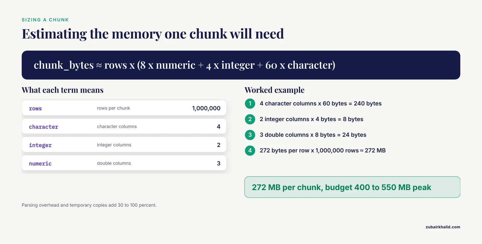
Estimate the in-memory size of one chunk before you run anything:
chunk_bytes ≈ rows x (8 x numeric columns + 4 x integer columns + 60 x character columns)The 60 bytes per character value accounts for R's per-string overhead (a pointer plus the string itself). For the file from Step 1, one million rows cost:
4 character columns x 60 bytes = 240
2 integer columns (pos, n) x 4 bytes = 8
3 double columns (beta, se, pvalue) x 8 bytes = 24
272 bytes per row x 1,000,000 rows ≈ 272 MB
Parsing overhead and temporary copies typically add 30 to 100 percent, so budget roughly 400 to 550 MB of peak RAM per one-million-row chunk. On a 16 GB machine that is comfortable. On an 8 GB machine shared with other jobs, drop to 200,000 rows per chunk, roughly 80 to 110 MB peak.
Two rules keep chunking stable. First, keep peak chunk memory under about 10 to 20 percent of available RAM so the operating system, R itself, and your accumulated results all fit. Second, divide your Step 1 row count by the chunk size to predict the loop count. At one million rows per chunk, the example file needs 29 chunks (28,122,709 divided by 1,000,000, rounded up).
Step 3: Chunk a Delimited File With data.table::fread
This loop is the template for most text-based genomic formats, including summary statistics and dosage files. Swap the filter line for your own per-chunk work and everything else stays the same:
library(data.table)

file_path    <- "gwas_sumstats.txt"
out_path     <- "gwas_hits.tsv"
chunk_rows   <- 1000000L

sumstats_names <- c("chrom", "pos", "snpid", "a1", "a2", "n",
                    "beta", "se", "pvalue")
sumstats_types <- c("character", "integer", "character", "character",
                    "character", "integer", "double", "double", "double")

## Fresh output file with a header
writeLines(paste(sumstats_names, collapse = "\t"), out_path)

skip        <- 1L     # line 1 is the header, start reading at line 2
n_processed <- 0L
n_hits      <- 0L

repeat {
  chunk <- fread(file_path, skip = skip, nrows = chunk_rows,
                 header = FALSE, colClasses = sumstats_types,
                 nThreads = 4L)
  if (nrow(chunk) == 0L) break
  setnames(chunk, sumstats_names)

  ## Per-chunk job: keep suggestive hits
  hits <- chunk[pvalue < 1e-5]
  if (nrow(hits) > 0L) {
    fwrite(hits, out_path, append = TRUE, sep = "\t", col.names = FALSE)
    n_hits <- n_hits + nrow(hits)
  }

  n_processed <- n_processed + nrow(chunk)
  skip <- skip + nrow(chunk)
  rm(chunk, hits)
}

cat("rows processed:", n_processed, "\n")
cat("hits kept:", n_hits, "\n")
Expected output:
rows processed: 28122709
hits kept: 6412
The parameters that matter:
skipandnrowsdefine the chunk window.skip = 1Lstarts after the header, and each iteration advancesskipby the rows actually read, which handles a short final chunk correctly.header = FALSEprevents fread from treating the first data row of each chunk as a header.colClassesfixes column types. Without it, fread guesses types per chunk, and a column that happens to hold whole numbers in one chunk reads as integer while the same column reads as double elsewhere.setnamesrenames columns by reference, which copies nothing.fwritewithappend = TRUEstreams results to disk instead of accumulating them.rm()releases each chunk promptly between iterations.
One honest caveat. fread implements skip by scanning and discarding lines, so each call re-reads the file from the top. With 29 chunks the example file gets read about 15 times in total. On a fast NVMe drive that adds a couple of minutes. On network storage it hurts, and you should prefer the streaming approach in Step 4 or split the file once up front with split -l 1000000.
Step 4: Stream a Delimited File With readr Chunked Callbacks
read_delim_chunked reads sequentially with no rescans, which makes it the better default when you have many chunks or slow storage. You supply a callback function that receives each chunk:
library(readr)

keep_hits <- function(chunk, pos) {
  chunk[chunk$pvalue < 1e-5, c("chrom", "pos", "snpid", "pvalue")]
}

hits <- read_delim_chunked(
  "gwas_sumstats.txt",
  delim = "\t",
  callback = DataFrameCallback(keep_hits),
  chunk_size = 100000,
  col_types = cols(chrom = col_character(), pos = col_integer(),
                   snpid = col_character(), a1 = col_character(),
                   a2 = col_character(), n = col_integer(),
                   beta = col_double(), se = col_double(),
                   pvalue = col_double()),
  progress = FALSE
)

nrow(hits)
#> [3] 6412
head(hits, 3)
#> # A tibble: 3 x 4
#>   chrom       pos snpid        pvalue
#>   <chr>     <int> <chr>         <dbl>
#> 1 2       2278969 rs7535560   4.1e-7
#> 2 6      32587410 rs9268877   2.3e-9
#> 3 9     136153924 rs10974440  9.7e-6
Parameter notes:
chunk_sizeis rows per chunk. Smaller chunks mean lower memory and more callback overhead.DataFrameCallbackcollects whatever the callback returns and binds it at the end. Use it when the kept result is small, as here.SideEffectCallbackignores return values. Use it when each chunk's output must go straight to disk because the kept set is large.col_typesplays the same role ascolClassesin fread, pinning types across chunks.progress = FALSEkeeps logs clean in scripts.
A third option for tabular data is arrow, which reads files in automatic batches and lets dplyr push the filter down:
library(arrow)
library(dplyr)

ds   <- open_dataset("gwas_sumstats.txt", format = "tsv")
hits <- ds |>
  filter(pvalue < 1e-5) |>
  select(chrom, pos, snpid, pvalue) |>
  collect()
Arrow suits the case where you will run many different filters against the same file. Converting once to parquet makes those repeated passes faster still.
Step 5: Chunk a VCF With the Bioconductor VariantAnnotation Package
This part of the guide works as a short Bioconductor tutorial for variant-level work. First compress and index the VCF (Variant Call Format, the standard text format for variant calls) so that block reading and later range queries are possible:
bgzip -c cohort.vcf > cohort.vcf.gz
tabix -p vcf cohort.vcf.gz
Then iterate with a yieldSize, which caps how many records each read returns:
library(VariantAnnotation)

vcf <- VcfFile("cohort.vcf.gz", yieldSize = 50000L)
open(vcf)

n_variants   <- 0L
n_missing_gt <- 0L

repeat {
  chunk <- readVcf(vcf, genome = "GRCh38",
                   param = ScanVcfParam(fixed = c("CHROM", "POS", "ID"),
                                        geno = "GT", info = NA))
  if (nrow(chunk) == 0L) break

  ## Per-chunk job: count missing genotype calls
  gt <- geno(chunk)$GT
  n_missing_gt <- n_missing_gt + sum(rowSums(gt == "./." | gt == ".|."))
  n_variants   <- n_variants + nrow(chunk)
}

close(vcf)
cat("variants:", n_variants, "\n")
cat("missing genotype calls:", n_missing_gt, "\n")
Expected output:
variants: 8421931
missing genotype calls: 1204817
Parameter notes:
yieldSizebounds memory per call. EachreadVcfcall advances the file handle, and an empty result ends the loop.ScanVcfParamis where the real savings live.fixedselects which fixed fields (CHROM, POS, ID, REF, ALT, QUAL, FILTER) to parse,genoselects genotype fields, andinfo = NAdrops all INFO annotations. Parsing only what you need often cuts memory by an order of magnitude.- Inspect one chunk before writing logic.
geno(chunk)$GT[1:5, 1:5]shows the missing-value notation your caller uses, which varies between./.,., and partially missing calls.
For cohort-scale work where you need the full genotype matrix repeatedly, convert the VCF to GDS (Genomic Data Structure) format with the Bioconductor SeqArray package, which applies functions over variant windows without loading the file.
Step 6: Chunk a BAM File With Rsamtools
BAM (Binary Alignment Map) files store aligned sequencing reads. The same yieldSize pattern applies:
library(Rsamtools)
library(GenomicAlignments)

bam <- BamFile("tumor.sorted.bam", yieldSize = 1000000L)
open(bam)

total_reads <- 0L

repeat {
  reads <- readGAlignments(
    bam,
    param = ScanBamParam(flag = scanBamFlag(isUnmappedQuery = FALSE))
  )
  if (length(reads) == 0L) break

  ## Per-chunk work goes here, for example tabulating
  ## alignments per chromosome or counting overlaps
  total_reads <- total_reads + length(reads)
}

close(bam)
total_reads
#> [3] 41283765
Parameter notes:
yieldSizeon theBamFileobject controls the read block, here one million alignments per call.ScanBamParamfilters and trims before data reaches R. Theflagargument here drops unmapped reads at the C level, and awhatargument can limit which fields (for examplec("rname", "mapq")) are extracted at all.readGAlignmentsreturns a compact object, so a million reads per chunk is a modest memory footprint.
The GenomicFiles package provides reduceByYield, which packages this read-combine loop so you supply only the per-chunk function and a combining rule. For gene-level counting specifically, GenomicAlignments::summarizeOverlaps with a BamFileList and yieldSize extends the same idea across many samples.
Step 7: Work Through a PLINK Genotype Matrix in SNP Blocks
PLINK binary genotype files (the .bed/.bim/.fam trio, unrelated to BED genomic intervals) are the standard container for cohort genotypes. The BEDMatrix package opens the .bed file as a file-backed matrix, so RAM use stays near zero until you extract a block:
library(BEDMatrix)

G <- BEDMatrix("cohort.bed")
dim(G)
#> [3] 500000  10000
Rows are SNPs and columns are individuals. Values are 0, 1, 2, or NA. Now loop over SNP blocks, compute per-SNP statistics, and write them into an HDF5 file as you go:
library(rhdf5)

n_snps     <- nrow(G)
block_size <- 2000L

h5createFile("snp_stats.h5")
h5createDataset("snp_stats.h5", "maf",          dims = n_snps, storage.mode = "double")
h5createDataset("snp_stats.h5", "missing_rate", dims = n_snps, storage.mode = "double")

for (start in seq(1L, n_snps, by = block_size)) {
  end   <- min(start + block_size - 1L, n_snps)
  block <- G[start:end, ]   # 2000 SNPs x 10000 individuals, about 160 MB

  allele_freq <- colMeans(block, na.rm = TRUE) / 2
  maf         <- pmin(allele_freq, 1 - allele_freq)
  missing     <- rowMeans(is.na(block))

  h5write(maf,     "snp_stats.h5", "maf",          index = list(start:end))
  h5write(missing, "snp_stats.h5", "missing_rate", index = list(start:end))
}

maf_all <- h5read("snp_stats.h5", "maf")
head(round(maf_all, 3))
#> [3] 0.247 0.499 0.132 0.381 0.004 0.296
Notes on this pattern:
- A 2,000-SNP block for 10,000 individuals is 20 million doubles, about 160 MB. Scale
block_sizeto your RAM using the Step 2 formula. colMeans(block) / 2gives the frequency of whichever allele BEDMatrix counts. Check the.bimfile to know which allele that is before labeling results.- The
indexargument inh5writewrites each block into its correct slice of the dataset, so the final file is complete and ordered. - The HDF5Array and DelayedArray Bioconductor classes read such files back in blocks with familiar matrix syntax.
Many cohorts distribute imputed dosages, the expected allele counts between 0 and 2 used for association testing, as plain text files [6]. The fread and readr loops from Steps 3 and 4 apply directly. The bigmemory package offers a related option for matrices you will revisit across sessions: read.big.matrix converts a text file once into a binary file-backed matrix, and later sessions attach to its descriptor file without re-parsing.
Step 8: Parallelize Chunks With BiocParallel
Chunks are embarrassingly parallel as long as each worker returns a small summary. BiocParallel distributes chunk start positions across workers:
library(BiocParallel)

n_data_rows <- 28122709L
chunk_rows  <- 1000000L
starts      <- seq(2L, n_data_rows + 1L, by = chunk_rows)  # data starts at line 2

hits_per_chunk <- bplapply(starts, function(start) {
  chunk <- fread(file_path, skip = start, nrows = chunk_rows,
                 header = FALSE, colClasses = sumstats_types)
  setnames(chunk, sumstats_names)
  nrow(chunk[pvalue < 1e-5])
}, BPPARAM = MulticoreParam(workers = 4L))

total_hits <- sum(unlist(hits_per_chunk))
total_hits
#> [3] 6412
Three constraints keep this safe:
- Memory multiplies by worker count. Four workers each holding a 400 MB chunk need about 1.6 GB plus overhead before results.
- Each worker rescans the file up to its
skipposition, so parallelskip-based reads multiply the scanning cost of Step 3. On slow storage, split the file once and give each worker its own file instead. - Workers must never append to one shared output file concurrently. Return summaries (as here) or write one file per worker and combine afterward.
MulticoreParamforks on Unix systems. On Windows, useSnowParam(workers = 4L).
Step 9: Write Results Incrementally
Three write patterns cover essentially every chunked job:
- Append inside the loop (Step 3). Simplest, and correct when the per-chunk output is a small filtered table.
- One file per chunk, combined at the end. Restart-friendly, because a crashed run leaves completed parts on disk:
part_dir <- "chunks"
dir.create(part_dir, showWarnings = FALSE)

## inside the loop
fwrite(hits, file.path(part_dir, sprintf("part_%03d.tsv", start)), sep = "\t")

## after the loop
final_hits <- rbindlist(lapply(list.files(part_dir, full.names = TRUE), fread))- HDF5 datasets written by index (Step 7). The right choice for numeric arrays you will read again in blocks.
The rule behind all three is the same: never accumulate full chunks in an R object across iterations. Accumulate only summaries, or write to disk and let the file system hold the bulk.
Step 10: Verify the Chunked Run
A chunked script that runs is not a chunked script that is right. Run four checks before you trust the output.
Row count. The processed count plus one header line must equal the wc -l total from Step 1. For the example, n_processed must print 28,122,709 against 28,122,710 total lines.
Column-sum cross-check. Accumulate one numeric column inside the loop and compare against an independent awk pass over the raw file. Column 8 is se:
awk -F'\t' 'NR > 1 {s += $8} END {printf "%.4f\n", s}' gwas_sumstats.txt
#> 4217481.3352
## inside the chunk loop
running_se_sum <- running_se_sum + sum(as.numeric(chunk$se))Agreement to four decimals confirms no rows were dropped, duplicated, or misparsed.
Header duplication. A common off-by-one bug writes the header row as data:
grep -c "^chrom" gwas_hits.tsv
#> 1
Any value above 1 means your skip arithmetic is wrong.
Spot check against a full in-memory load. On a truncated copy of the file, run the same filter with a plain in-memory fread and compare row counts and a few rows against the chunked output. This catches type mismatches and boundary errors that row sums miss:
sample_rows <- read.delim("gwas_sumstats.txt", skip = 5000000, nrows = 1000,
                          header = FALSE, sep = "\t")
names(sample_rows) <- sumstats_names
kept <- sample_rows[sample_rows$pvalue < 1e-5, ]

hits_tbl <- fread("gwas_hits.tsv")
sum(kept$snpid %in% hits_tbl$snpid) == nrow(kept)
#> [3] TRUE
Finish with md5sum gwas_hits.tsv so the exact output version is recorded for reproducibility.
Which Approach to Use When
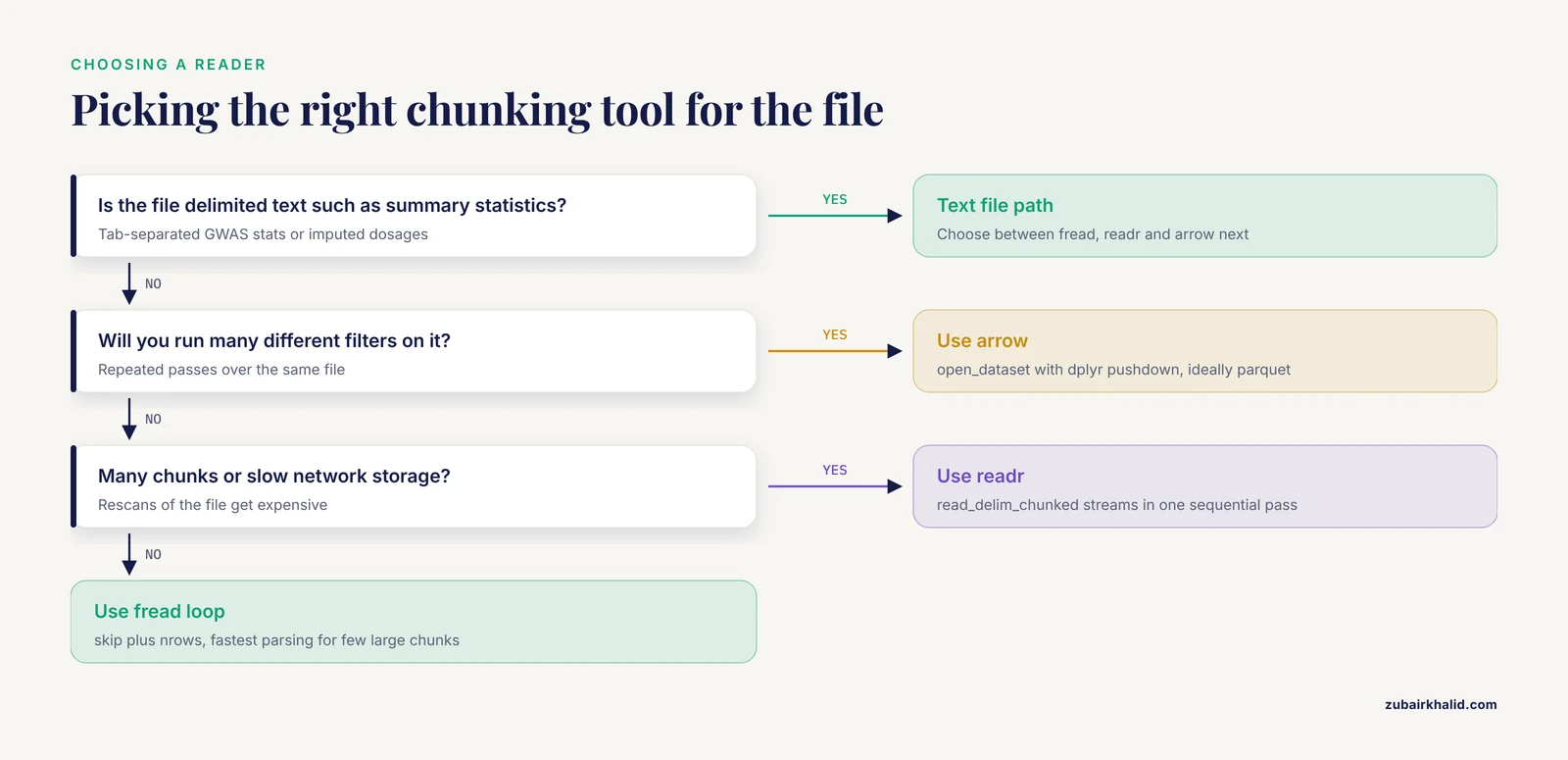
| Situation | Tool | How chunks are controlled | Memory profile |
|---|---|---|---|
| Delimited text, few large chunks, fastest parsing | data.table::fread loop | skip + nrows | One chunk in RAM, rescans on each skip |
| Delimited text, many chunks or slow storage | readr::read_delim_chunked | chunk_size + callback | One chunk in RAM, single sequential pass |
| Repeated filters or column subsets on tabular data | arrow::open_dataset | Automatic batches | Batches, dplyr pushdown |
| VCF or BCF, variant-level work | VariantAnnotation::readVcf | VcfFile(yieldSize) | One variant block in RAM |
| BAM or CRAM, read-level work | Rsamtools + GenomicAlignments | BamFile(yieldSize) | One read block in RAM |
| PLINK binary genotype matrix | BEDMatrix | SNP-row block indexing | File-backed, near-zero RAM |
| Reusable on-disk numeric matrix | bigmemory, HDF5Array, rhdf5 | Explicit block index | File-backed |
| Large cohort VCF, many samples | SeqArray (GDS) | Variant windows | File-backed |
Once a chunked script works, wrap it rather than copy it. Keep the loop as a function that takes a path, a chunk size, and a processing function, and log per-chunk counts to a run log. Teams that manage many such scripts organize them into pipelines with tracked dependencies between steps, which is the design behind platforms like CoreFlow [7]. When results need to reach collaborators, attach a dashboard layer to the same pipeline instead of emailing static plots, the use case i2dash was built for in large-scale sequencing facilities [8]. And when an analysis area matures, look for a package that already implements the scale engineering for you, the way coADAPTr automated high-throughput covalent labeling analysis in R [9] and LT-FGRS brought population-scale family-based liability estimation to a manageable computational cost [10].
Common Mistakes and Limitations
- Growing results inside the loop.
results <- rbind(results, chunk)copies the whole object on every iteration, quadratic cost that ends inError: cannot allocate vector of size 3.5 Gb. Write incrementally or collect small summaries in a preallocated list. - Off-by-one in skip arithmetic. Symptoms are a header line parsed as data (type errors on the first chunk) or a silently lost first data row. Always test on a 10,000-row file where you can eyeball the output before scaling up.
- Per-chunk type guessing. Both fread and readr infer types within a chunk. A
pvaluecolumn that happens to hold whole numbers in one chunk reads as integer and breaks the final bind. Always passcolClassesorcol_types. - Ragged rows. fread reports
Stopped early on line 2000001. Expected 9 fields but found 8.and read.table reportsline 2000001 did not have 9 elements. Locate the offending lines with the awk field-count check from Step 1, fix upstream, or usefill = TRUEin read.table and then verify what got filled. Never let silent filling into a results file. - Statistics that need global context. Filtering, counts, sums, and running means stream perfectly. Quantiles, genome-wide LD pruning, and anything requiring globally sorted order do not. Plan two-pass designs: pass one accumulates sufficient statistics, pass two applies thresholds.
- Parallel workers multiplying memory and rescans. Four workers each holding a large chunk, each rescanning the file to its skip position, can saturate both RAM and a shared filesystem. Return small summaries from workers.
- Unclosed connections. Loops that open files without
on.exit(close(con), add = TRUE)eventually fail withcannot open the connectionandToo many open files. Close what you open, every time. - Integer overflow. Summing a large integer column prints
NAs produced by integer overflowbecause R integers cap at 2^31 minus 1. Wrap the column withas.numeric()before summing. - Out-of-memory kills leave no R error. The session vanishes, RStudio reports
R Session Aborted, and the terminal printsKilled. Check system logs (dmesg | grep -i oom) and reducechunk_rows. Callingrm()andgc()between chunks helps long sessions. - R is not always the right layer.
bcftools,plink2, andawkfilter single-pass files faster than any R loop. Purpose-built tools exist for good reasons: gJLS2 is designed to be called from PLINK for biobank-scale genome-wide analysis [11], BESSiE moved large-scale Bayesian marker analyses out of pure R [3], and PRSice-2 exists because biobank-scale PRS computation demands more efficiency than general environments provide [4]. Use R for statistics, visualization, and glue, and hand raw-scale filtering to compiled tools. - Missing-data discipline. Define NA handling once per pipeline and never drop it silently. Large-scale quantitative studies show missingness patterns can differ systematically across batches, which is why methods like SALPS model missing peptide intensities explicitly rather than discarding them [12]. The same discipline applies to genotype missingness and low-coverage metrics.
- HPC mapping. Chunked R scripts map naturally onto scheduler array jobs, one task per chunk range. ascatNgs documents both one-shot execution and approaches suitable for large-scale compute farms for exactly this reason [13].
Frequently Asked Questions
How big does a file need to be before chunking is necessary in R?
Chunk once the fully loaded object would exceed roughly a quarter of your available RAM. Estimate this by multiplying rows by bytes per row (8 for doubles, 4 for integers, about 60 for character values), then add 30 to 100 percent for parsing overhead.
What chunk size should I use?
Start at 100,000 to 1,000,000 rows for text files, or 10,000 to 50,000 records for VCF and BAM files, then adjust against measured peak memory. Keep peak chunk memory near 10 to 20 percent of RAM so results and the operating system fit alongside it.
Do I need to convert my VCF before chunked processing in R?
No. VariantAnnotation reads chunked VCFs directly once the file is bgzip-compressed and tabix-indexed. For repeated passes over a large cohort, converting once to GDS with SeqArray or to BCF pays for itself.
Can I run chunked processing in parallel in R?
Yes. BiocParallel's bplapply over chunk start positions works well when each worker returns a small summary. Watch for memory multiplication by worker count, repeated skip rescans, and concurrent writes to one shared output file.
How do I handle ragged or inconsistent columns?
Find the bad lines first with an awk field-count check, then fix the file upstream or read with fill = TRUE and verify what was filled. Silent filling in a genomic results file is a data integrity problem, not an inconvenience.
Should I use data.table, readr, or arrow for chunked text files?
Use readr for strict streaming with many chunks or slow storage, data.table's fread for the fastest parsing with few large chunks, and arrow when you will run many different filters against the same file, ideally after converting to parquet.
How do I write chunked results without running out of memory?
Append each chunk's output to disk inside the loop, or write one small file per chunk and combine at the end, or write numeric arrays into indexed HDF5 datasets. Never accumulate full chunks in a list unless the kept result is provably small.
When should I move the work out of R entirely?
When a single-pass filter or format conversion dominates runtime, hand it to bcftools, tabix, or plink2 and bring only the reduced data into R. R earns its keep on modeling, statistics, and visualization, not on brute-force file filtering.
Sources
- Towards computational solutions for precision medicine based big data healthcare system using deep learning models: A review.
- CANEapp: a user-friendly application for automated next generation transcriptomic data analysis.
- BESSiE: a software for linear model BLUP and Bayesian MCMC analysis of large-scale genomic data.
- PRSice-2: Polygenic Risk Score software for biobank-scale data.
- GWAtoolbox: an R package for fast quality control and handling of genome-wide association studies meta-analysis data.
- Using imputed genotype data in the joint score tests for genetic association and gene-environment interactions in case-control studies.
- CoreFlow: a computational platform for integration, analysis and modeling of complex biological data.
- i2dash: Creation of Flexible, Interactive, and Web-based Dashboards for Visualization of Omics Data.
- Covalent Labeling Automated Data Analysis Platform for High Throughput in R (coADAPTr): A Proteome-Wide Data Analysis Platform for Covalent Labeling Experiments.
- LT-FGRS: a unifying R-package for the estimation of family-based genetic liabilities at population-scale.
- gJLS2: an R package for generalized joint location and scale analysis in X-inclusive genome-wide association studies.
- Detecting differential protein expression in large-scale population proteomics.
- ascatNgs: Identifying Somatically Acquired Copy-Number Alterations from Whole-Genome Sequencing Data.