Bulk vs Single-Cell RNA-seq Normalization: Why Your Go-To Methods Fail

Q: When should I use bulk instead of single-cell approaches?

Use bulk when your question concerns average expression across a tissue, when you need statistical power from many biological replicates, or when your input is already aggregated. Use single-cell when cell-type identity, state transitions, or rare populations are the question. Many projects use both, bulk for cohort-level statistics and single-cell for cellular interpretation.

By Dr. Zubair Khalid, DVM, MS, PhD · 2026-11-11

Bulk vs Single-Cell RNA-seq Normalization: Why Your Go-To Methods Fail

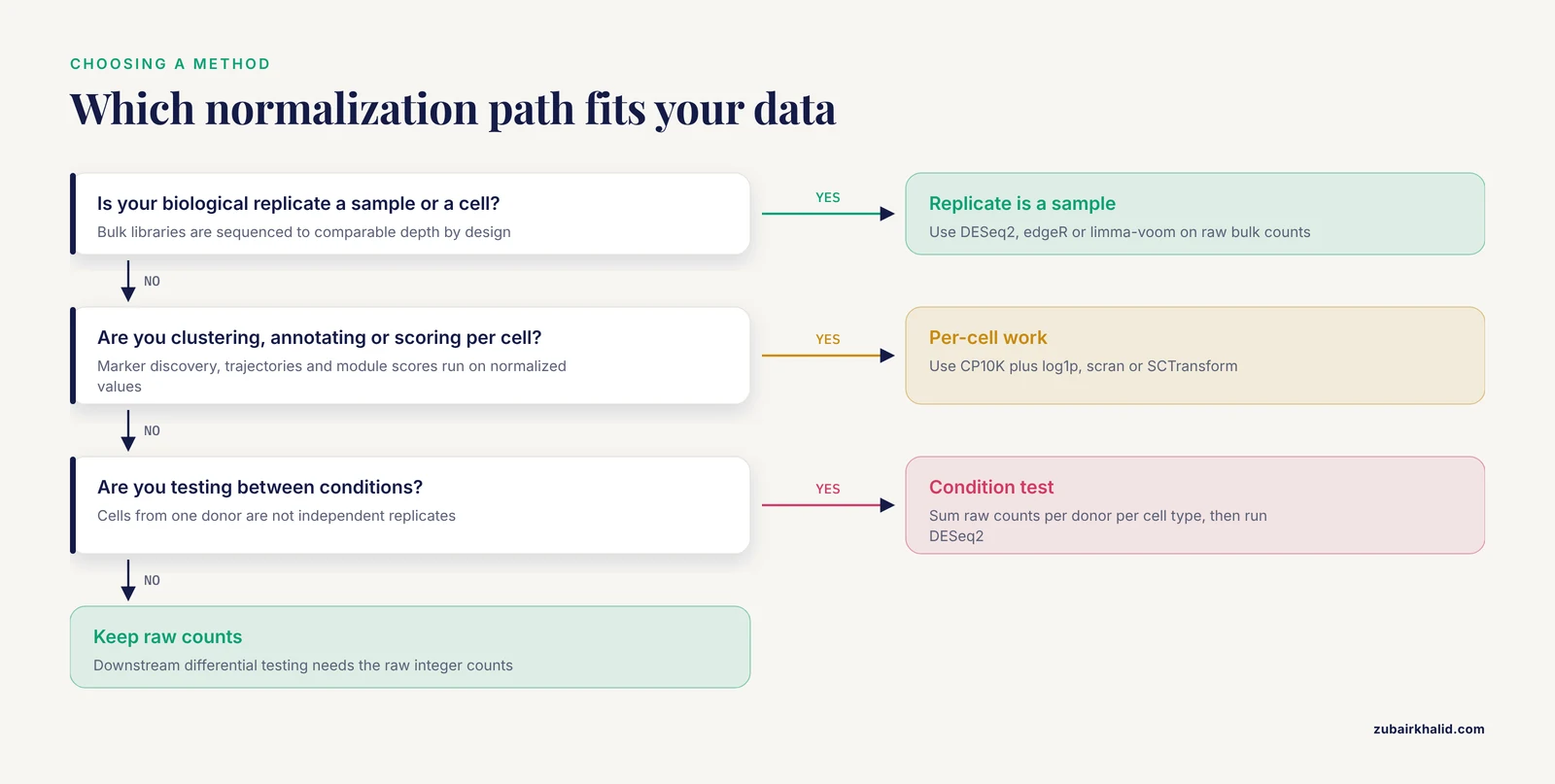
Bulk RNA-seq normalization scales counts to make whole-tissue libraries comparable, while single-cell normalization must additionally cope with extreme sparsity, wildly varying sequencing depth per cell, and a count distribution that standard bulk models do not describe. The rule of thumb is simple: if your biological replicate is a sample, use a bulk method such as DESeq2, edgeR, or limma-voom on aggregated counts. If your biological replicate is a cell within a donor, use a single-cell method for exploratory work, but switch to pseudobulk aggregation whenever you test differential expression between conditions.

This article explains the difference between bulk and single cell RNA-seq normalization, shows why each method breaks when applied to the wrong data type, and gives you a decision framework plus worked scenarios you can copy into your own pipeline.

The One-Sentence Difference and the Rule of Thumb

Decision path asking whether replicates are samples or cells, leading to bulk tools, per-cell normalization or pseudobulk.

Bulk normalization answers one question: how do I make the total read counts of a handful of samples comparable so that gene-level differences reflect biology rather than sequencing depth? Single-cell normalization answers a harder question: how do I make tens of thousands of sparse count vectors comparable to each other without letting sequencing depth or technical dropout masquerade as biology?

The rule of thumb for choosing between bulk or single-cell RNA-seq normalization:

Differential expression between conditions with real biological replicates? Aggregate cells into pseudobulk per donor and cell type, then run a bulk pipeline. Recent integrative studies do exactly this, using patient-level pseudobulk differential expression as the core test rather than cell-level tests [1].
Clustering, marker discovery within a sample, trajectory inference, or annotation? Per-cell normalization such as log-normalization or SCTransform is appropriate.
Reusing a published single-cell dataset to strengthen a bulk finding, or validating bulk biomarkers at single-cell resolution? Normalize each dataset on its own terms first, then integrate. Many recent cancer and disease studies follow this pattern, screening bulk candidates and then checking where those genes are expressed at the cellular level [2], [3], [4].

If you take one sentence from this article: never judge a single-cell result with a bulk statistic, and never judge a bulk result with a single-cell visualization.

What Bulk Normalization Actually Does

In bulk RNA-seq you sequence an entire tissue or cell population. Each library produces tens of millions of reads spread across roughly 20,000 genes, so most genes receive substantial counts. The data matrix is wide and shallow in one sense, with many samples but deep coverage per gene. Normalization methods fall into a few families.

Scaling methods: CPM, TPM, and their limits

Counts per million (CPM) divides each gene count by the library total and multiplies by one million. Transcripts per million (TPM) additionally divides by gene length, so TPM values are comparable across genes within a sample. These are descriptive scaling methods. They are fine for plots, sample-level correlation heatmaps, and method comparisons such as the single-sample network evaluations that took transcriptomic profiles from cancer cell line databases as their input [5].

Where these methods fail is differential expression. CPM and TPM have no model for sampling variance. A gene with a count of 5 in one sample and 15 in another has the same threefold ratio whether the counts are 5 and 15 or 500 and 1,500, but the statistical evidence is completely different. Bulk differential expression methods model the count itself.

Model-based methods: DESeq2, edgeR, and limma-voom

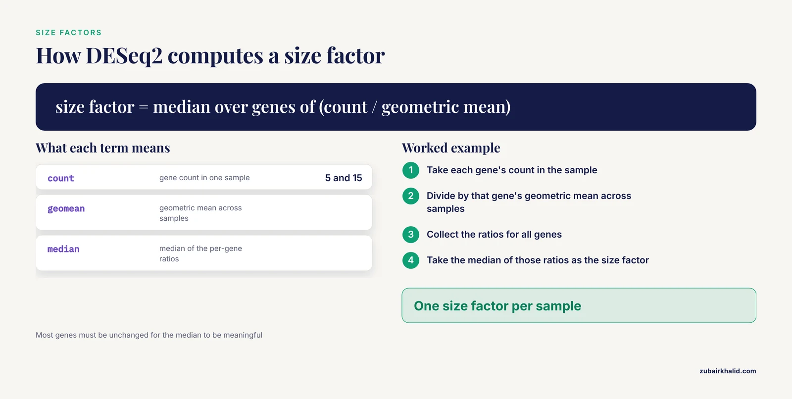
Worked median-of-ratios example with gene ratios against geometric means and the median size factor.

DESeq2 and edgeR use negative binomial generalized linear models on raw counts, estimating a dispersion parameter per gene. DESeq2 computes size factors with the median-of-ratios method. For each gene, you calculate the ratio of its count in a sample to its geometric mean count across samples, then take the median of those ratios as the sample's size factor. This assumes most genes are not differentially expressed, which is usually reasonable and is precisely the assumption naive CPM normalization lacks when a few highly expressed genes dominate library composition.

edgeR uses trimmed mean of M values (TMM), which similarly trims extreme log-fold-change genes before computing scaling factors. limma-voom transforms counts to a log-counts-per-million value with a precision weight per observation, then applies linear modeling. All three require raw counts as input, a design matrix with biological replicates, and moderate per-gene counts to estimate dispersion.

These methods are mature, well documented, and remain the standard for bulk differential expression. Every recently published integrative workflow in the literature that analyzed bulk RNA-seq data used a variant of this approach, with paired designs, within-patient comparisons, and false discovery rate correction [1].

Why bulk normalization fails on single-cell data

Take a typical 10x Genomics matrix. A cell with 30,000 reads has counts for maybe 1,000 to 3,000 genes. Over 80 percent of the matrix is zero. Now apply median-of-ratios size factors per cell:

The geometric mean across cells for most genes is zero, so the ratio for that gene is undefined and gets filtered. In deep dropout, many cells lose so many genes that the size factor becomes unstable or zero.
Negative binomial dispersion estimation per gene is impossible when nearly all observations are zero. The model has nothing to estimate from.
The resulting size factors become a function of how many genes happened to be captured, which is confounded with cell type. Small immune cells capture fewer genes than large epithelial cells. A size factor "correcting" that difference can erase a real biological difference in RNA content.

This is the first major rna seq error researchers hit when moving from bulk to single cell: the tool that always worked suddenly produces nonsense, not because the tool is wrong but because the data violate its assumptions.

What Single-Cell Data Breaks

The difference between bulk and single cell RNA-seq normalization comes down to three properties of the count matrix.

Sparsity and dropout

In bulk data, zeros usually mean "not expressed" or "below detection," and they are rare for moderately expressed genes. In single-cell data, zeros dominate because of low capture efficiency and shallow sequencing per cell. A gene expressed at a steady level in every cell of a type can still show 60 percent zeros in a droplet-based dataset. This is dropout, the technical absence of a count for a transcript that was present.

Dedicated single-cell methods exist because of this. The scGSCA framework was built specifically because bulk gene-set co-expression methods do not handle sparse counts, single-cell distributional noise, subject-level dependence, and cell-type heterogeneity. Its authors fit gene-wise zero-inflated negative binomial mixed models with subject-level random effects and compute statistics on quantile residuals, a design that would be pointless if bulk-style normalization carried over cleanly [6].

Library size variation across orders of magnitude

Within a single 10x run, total UMI counts per cell can range from 1,000 to 50,000 or more. Part of this is technical, sequencing depth, and part is biological, RNA content per cell. Bulk data never face this problem because every library is sequenced to a comparable depth by design. Single-cell normalization must decide how much of the depth difference to remove. Removing all of it can wash out genuine cell-size and cell-cycle biology. Removing none of it makes every downstream analysis a proxy for sequencing depth.

No true replication at the cell level

Cells from the same donor are not independent. A differential expression test that treats 5,000 cells from one patient as 5,000 replicates will produce tiny p-values for any difference between two donors, because it mistakes sample identity for biological signal. This is the single most common rna seq error in published single-cell analyses and the reason several recent papers explicitly use the donor as the biological replicate and analyze cell-level data with donor-aware models [7].

The consequence for normalization is subtle but real. Normalization choices that seem purely technical, such as how aggressively you scale library sizes, change cell-level scores, and cell-level scores feed cluster assignments, which feed the pseudobulk aggregation that the valid statistical test ultimately uses. Errors upstream propagate.

How Single-Cell Normalization Actually Works

Log-normalization: CP10K plus log1p

The default in Scanpy and Seurat is a two-step recipe. First, scale each cell's counts to a fixed total, commonly 10,000, which gives counts per 10,000 (CP10K). Second, apply log1p, the natural logarithm of the value plus one. The plus one handles zeros.

In Scanpy this is two lines:

sc.pp.normalize_total(adata, target_sum=1e4)
sc.pp.log1p(adata)

In Seurat the equivalent is NormalizeData() with the default LogNormalize method. The result is a roughly symmetric distribution that works well for PCA, neighborhood graphs, UMAP, and Leiden clustering, which is exactly the pipeline described in a recent osteosarcoma single-cell study that retained 44,189 cells and 25,473 detected genes after quality control [8]. The same log-normalization step appears in standard single-nucleus workflows built on Seurat [9].

Log-normalization is a workhorse, not a model. Its known weaknesses:

The target sum (10,000 versus a million) changes the compression of the data and can change downstream results.
The log transform is applied to scaled counts whose noise structure does not match the transform, so highly expressed genes and lowly expressed genes are treated with the same variance stabilization, which is wrong for both.
Differences in total RNA content between cell types are partially or fully removed depending on implementation, which can shift apparent cell identities.

scran pooling and size factors with shrunken variance

scran addresses unstable per-cell size factors by pooling cells, computing size factors on pools where counts are less sparse, and deconvolving back to per-cell factors. This produces more stable size factors for very sparse data, especially Smart-seq2-style full-length data with low cell numbers. It remains a solid choice when you need per-cell size factors that behave more like bulk size factors.

SCTransform and regularized negative binomial regression

SCTransform, the default normalization in Seurat workflows for many labs, fits a regularized negative binomial model of UMI counts with sequencing depth as a covariate, then regresses out technical variation and returns Pearson residuals. The idea is to model the count-generating process rather than apply a fixed transform. It tends to produce cleaner clustering on droplet data and handles the depth-confounding problem more explicitly than CP10K plus log1p.

The caveat is that SCTransform residuals are not counts and not log-expression. Feeding them into tools that expect either is a classic troubleshooting trap. Differential expression on SCTransform output requires methods designed for it, or better, a return to raw counts and pseudobulk.

Platform scale differences are not a normalization problem you can ignore

Smart-seq2 and 10x produce data on different effective scales. Smart-seq2 is full-length and deeper per cell, 10x is droplet-based and shallower with many more cells. A recent glioblastoma study that analyzed deposited Smart-seq2 and 10x matrices from the same public resource explicitly audited each dataset on its verified expression scale before any integration, and excluded alias-affected records from score denominators [10]. The practical lesson: before normalizing a merged dataset, confirm that every matrix is in the same unit, raw counts or processed values, and re-derive normalization per platform if they differ. Failing this check is one of the most common bioinformatics troubleshooting issues when combining public data.

Pseudobulk: The Bridge Between the Two Worlds

Pseudobulk aggregation sidesteps most of the normalization conflict. You sum raw counts of all cells of a given cell type within a given donor, producing one count vector per donor per cell type. That vector looks exactly like a bulk RNA-seq library, with realistic counts and realistic dispersion, and you can run DESeq2 or edgeR on it with donor as the replicate.

This is what modern integrative studies do as a matter of course:

A colorectal cancer liver metastasis study retained 132,915 single cells after quality control and ran paired single-cell pseudobulk differential expression between primary tumors and matched metastases at the patient level, applying Benjamini-Hochberg false discovery rate correction across the gene set [1].
A membranous nephropathy study used the donor as the biological replicate across three kidney single-cell datasets and one bulk cohort, evaluating a 47-gene program with donor-level pseudobulk analysis plus leave-one-donor-out and leave-one-gene-out sensitivity analyses [7].
An endometrial carcinoma study built a 43,613-cell atlas, performed differential expression and hdWGCNA within an epithelial lineage, and used pseudobulk among its sensitivity analyses before prioritizing candidates against a bulk TCGA cohort [11].

Why pseudobulk beats cell-level differential testing for condition comparisons:

It restores the correct unit of replication, the donor, so p-values mean what they claim.
It recovers realistic count depth, so negative binomial models have something to estimate.
It sidesteps the log-normalization choice entirely, because DE happens on raw aggregated counts.
It is computationally trivial compared with per-cell mixed models over tens of thousands of cells.

The requirement is a design with enough donors per condition. Pseudobulk with two donors per condition is a descriptive comparison, not an inferential one, a limitation that recent immune-oncology reanalyses state openly when only one sample was available per response group [12].

Side-by-Side Comparison

Criterion	Bulk RNA-seq normalization	Single-cell RNA-seq normalization
Unit being normalized	One library, one tissue or population	One cell, one nucleus, or one pseudobulk aggregate
Typical counts per feature	Tens to thousands of reads per gene	Zero to a few hundred UMIs per gene per cell
Matrix density	Nearly dense	Often over 80 percent zeros
Library size spread	Similar across samples by design	Frequently 10-fold or more within one run
Core assumption	Most genes unchanged across samples	No assumption transferable from bulk, cell types differ in RNA content
Standard methods	DESeq2 median-of-ratios, edgeR TMM, limma-voom, CPM and TPM for description	CP10K plus log1p, scran pooled size factors, SCTransform regularized NB
Input for DE testing	Raw counts directly	Raw pseudobulk counts, or cell-level models built for sparse counts
Main failure mode	Compositional bias when many genes shift in one direction	Depth and dropout confounding, pseudo-replication of cells
Typical downstream goal	Sample-level signatures, biomarkers, prognostic models	Cell-type identification, state programs, trajectories
Aggregation is easy?	Already aggregated	Requires summing raw counts per donor per cell type before DE

When to Use Bulk Normalization

Use bulk methods, meaning DESeq2, edgeR, or limma-voom on raw counts, in these situations:

You have raw bulk count matrices with three or more biological replicates per condition and a design matrix. This remains the standard for tumor versus normal comparisons, and it is how recent sinonasal carcinoma work analyzed 14 bulk tumor and normal samples alongside single-nucleus data [13].
You have aggregated single-cell counts per donor per cell type. Pseudobulk DE is a bulk problem and bulk tools are the correct answer.
You are building sample-level signatures, co-expression modules, or prognostic models from cohort data, as in the weighted gene co-expression network analyses combined with LASSO Cox modeling on TCGA and GEO bulk cohorts in gastric cancer work [14].
You are computing gene-set or pathway scores that will be compared across samples.

Do not use bulk per-gene models cell by cell. The data are too sparse, the replicate structure is wrong, and the variance model does not fit.

When to Use Single-Cell Normalization

Use per-cell normalization in these situations:

Clustering and cell-type annotation. Every published workflow cited here performed quality control, normalization, dimensionality reduction, and Leiden clustering on per-cell normalized data [8], [9].
Marker gene discovery within a dataset, where you compare clusters of cells and rank genes by log fold change on normalized values.
Program and module scoring. AddModuleScore, UCell, AUCell, and similar scorers run on normalized log-scale data, and they are the standard way to transfer a bulk-derived gene list into cellular context [14], [15].
Trajectory and state analyses. Pseudotime, RNA velocity, and state scoring all operate on per-cell normalized values [16].

Do not use per-cell p-values for between-condition claims. A Wilcoxon test across cells answers "do these clusters differ," not "do these patients differ."

Worked Scenarios

Scenario 1: Validating a bulk biomarker at single-cell resolution

You find MARCKSL1 elevated in prostate tumor bulk RNA-seq and want to know which cells express it. The published prostate cancer study did exactly this, screening tumor-derived transcripts from bulk tissue and urine sequencing against single-cell datasets from normal prostate and prostate tumor tissues, then validating a candidate in urine qPCR [2]. The correct pipeline: normalize the bulk and single-cell datasets separately, on their own terms, map the bulk candidate onto the single-cell atlas using a module score on log-normalized data, and report which cell populations carry the signal. Normalizing the single-cell data with a bulk method first would have corrupted the cell-type assignment before any comparison happened.

Scenario 2: Differential expression from a single-cell experiment

You have 6 patients per condition, 10x data, and annotated cell types. The wrong way: subset the log-normalized matrix to epithelial cells, run a Wilcoxon test on 20,000 cells, and report p-values. The right way: go back to raw counts, sum them per donor per cell type, build a matrix with 12 rows (donors) and the gene columns, and run DESeq2 with a condition covariate. This is the patient-level pseudobulk design used in the colorectal liver metastasis analysis [1] and the donor-aware design in the kidney study [7]. If no gene survives FDR correction even in pseudobulk, as happened in that paired metastasis comparison, report it honestly rather than falling back to cell-level p-values that always look significant [1].

Scenario 3: Integrating public data from two platforms

You combine a Smart-seq2 cohort and a 10x cohort. The glioblastoma reanalysis offers the template: audit each dataset's expression scale before analysis, keep them on their verified scales, recompute states within each platform, and benchmark predictions against an independent bulk cohort such as TCGA [10]. Normalizing both datasets with the same function call without checking input units produces spurious platform clusters that look like biology.

Scenario 4: Pathway-level questions across cell types

You want to know whether a pathway's internal coordination, not just its average expression, differs between tumor and normal. Bulk gene-set methods on aggregated data lose the cellular context, and naive per-cell correlation is destroyed by sparsity and subject dependence. The scGSCA approach exists for this exact gap, fitting zero-inflated negative binomial mixed models and testing whether co-expression between two cell types varies by sample phenotype [6]. Its gastric cancer and breast cancer applications found pathway signals, including axon guidance and IL6-JAK-STAT3, that bulk analysis did not capture [6].

Scenario 5: Small targeted panels

Single-cell qPCR produces Ct values rather than counts, and normalization there is its own problem. The deltaXpress tool takes cycle threshold values, selects the best pair of housekeeping genes for normalization, and then supports both bulk-style differential expression comparisons and pairwise differentially correlated genes between conditions [17]. The lesson generalizes: normalization method must match the measurement scale, Ct values, UMIs, and read counts each need their own treatment.

Common Mistakes and Limitations

These are the failures seen most often in real pipelines, organized for practical bioinformatics troubleshooting.

Using TPM or log-normalized values as DESeq2 or edgeR input. Both tools require raw integer counts. Feeding them normalized floats silently disables the count model and invalidates dispersion estimates.

Treating cells as replicates. This is the most damaging error. A test across 30,000 cells from 3 donors has an effective sample size of 3 for between-donor questions. Donor-aware pseudobulk or mixed models with donor random effects are the fix, and the donor-as-replicate principle is now explicit in current multi-cohort workflows [7].

Normalizing before removing low-quality cells. Broken cells, empty droplets, and doublets distort size factors for every cell in the library. Quality control, ambient RNA correction, and doublet detection come first, and recent multi-layer reanalyses run rigorous QC and doublet detection before any downstream step [13].

Comparing fold changes across platforms without checking scale. A 10x UMI matrix and a Smart-seq2 read-count matrix quantify expression differently, and fold changes are not directly comparable until each is processed on its verified scale [10].

Mixing up what TPM means across genes and across cells. TPM is comparable for a single gene across cells, and comparable for genes within a single cell, but the two comparisons answer different questions and TPM has no role in statistical testing.

Assuming log1p makes distributions normal. It compresses but does not fix zero inflation. For inferential statistics on sparse data, use methods built for it, such as the zero-inflated negative binomial mixed modeling in scGSCA [6].

Overinterpreting single-sample comparisons. When a dataset contains one responder and one non-responder, every difference is descriptive, and recent endometrial cancer reanalyses label such comparisons hypothesis-generating for exactly this reason [12]. Pseudobulk cannot rescue a design with no replication.

Forgetting compositional effects in bulk. If one cell type doubles in tumor tissue, its genes appear upregulated in bulk even if per-cell expression is unchanged. This is why bulk hits need single-cell follow-up, and why single-cell-derived cell-type fractions improve the interpretation of bulk immune signatures, a pattern visible across the integrative oncology studies cited here [1], [15], [4].

Regressing out too much. Regressing library size, cell cycle, and mitochondrial fraction out of normalized data can remove real biology. Cell-cycle programs, for example, are often the strongest real signal in a tumor atlas and showed up as a cross-layer finding when single-nucleus and bulk data were reanalyzed together in sinonasal carcinoma [13]. Decide per covariate whether it is technical noise or signal.

Ignoring the aggregation step's inputs. Pseudobulk inherits every upstream error, wrong cell-type labels, uncorrected batch effects, ambient RNA. Sensitivity analyses such as leave-one-donor-out checks are cheap insurance and were used explicitly in the kidney pseudobulk workflow [7].

A final limitation applies to all of this: normalization choices change downstream results, and no single method is universally best. Report which normalization you used, run a sensitivity check with a second method when a result matters, and remember that any individual project decision benefits from consultation with a senior analyst or biostatistician before locking the pipeline.

Frequently Asked Questions

Can I run DESeq2 directly on a single-cell count matrix?

Not cell by cell. The matrix is too sparse for dispersion estimation, and the per-cell size factors that median-of-ratios produces are unstable when most genes are zero. Run DESeq2 on pseudobulk counts summed per donor per cell type instead, which restores realistic counts and the correct replicate structure.

What is the difference between bulk and single-cell RNA-seq normalization in one practical sense?

Bulk normalization corrects differences in total sequencing depth between a small number of deeply sequenced libraries. Single-cell normalization must also decide how much per-cell depth variation to remove, handle pervasive dropout, and avoid erasing real differences in RNA content between cell types, so the methods and their failure modes are genuinely different.

When should I use bulk instead of single-cell approaches?

Use bulk when your question is about average expression across a tissue, when you need statistical power from many biological replicates, when budget limits cell numbers, or when your input is already aggregated such as TCGA data. Use single-cell when cell-type identity, state transitions, or rare populations are the question. Many current projects use both, bulk for cohort-level statistics and single-cell for cellular interpretation [2], [3].

Why do my single-cell fold changes look smaller than bulk fold changes?

Per-cell log fold changes are computed on noisy, dropout-laden normalized values, which shrinks estimates, and bulk fold changes mix per-cell expression with shifts in cell-type composition. A bulk "upregulation" can be entirely compositional, which is why cell-type-resolved verification is now standard in integrative oncology analyses [1], [18].

Should I normalize before or after batch correction and integration?

Normalize first. Integration methods such as Seurat integration, Harmony, and scVI expect normalized input, usually log-normalized, and they correct batch effects in that space. Normalizing after integration re-introduces the depth and platform differences the integration was designed to remove.

Is SCTransform better than log-normalization?

For droplet-based data, SCTransform often produces cleaner clusters because it models the count-generating process and handles sequencing depth explicitly. For Smart-seq2 data, small datasets, or when you need counts for pseudobulk, log-normalization plus raw-count aggregation is simpler and sufficient. Whichever you choose, keep the raw counts in the object, because downstream differential testing will need them.