How to Build a Simple Bioinformatics Analysis Pipeline from Scratch

By Dr. Zubair Khalid, DVM, MS, PhD · 2026-11-11

By the end of this article you will have a working, reproducible bioinformatics analysis pipeline that takes paired-end FASTQ files as input, runs quality control, trims adapters, aligns reads to a reference genome, produces per-sample summary statistics, and rolls everything into a single QC report. You will build it as a plain shell script first, then see how the same logic translates into a Nextflow workflow, so the template scales from a laptop to a server without rewriting your science.

Here is what you need on hand before you start:

1. A computer with Linux, macOS, or the Windows Subsystem for Linux.
2. At least 16 GB of RAM and 100 GB of free disk space if you want to run a real dataset. A bacterial genome dataset works on a laptop, a human genome dataset wants a server.
3. Conda (Miniconda is enough) for installing tools.
4. A small test dataset. Two or three paired-end samples are plenty. If you do not have your own data, download a small FASTQ pair from a public repository such as SRA or ENA using the accession's FTP links.
5. A reference genome FASTA file for the organism you study.

Everything in this article is written so you can type it or paste it and get a concrete result. The directory layout, sample sheet, driver script, and Nextflow skeleton form a build bioinformatics pipeline from scratch template you can adapt to almost any sequencing assay, from RNA-seq to metagenomics to CUT&Tag.

Why the Template Design Matters More Than the Tools

Beginners usually ask which aligner to use. Experienced analysts ask a different question: how will someone else, or you in six months, rerun this analysis and get the same numbers? Reproducibility is the design constraint that shapes everything else.

Recent work makes this concrete. The SCRATCH pipeline for single-cell cancer research was built on Nextflow with a layered, modular architecture that follows FAIR principles and the guidelines of the nf-core community, precisely so that results do not change when a human intervenes at a different point [1]. The STATegra project took the same idea one level up and argued that multi-omics analyses should start from a written conceptual scheme, a stepwise plan for how data layers combine, before anyone picks a tool, because otherwise every study reinvents an ad hoc combination from zero [2]. Both papers describe the same habit: define the flow of data first, then wire tools into that flow.

A template enforces that habit. It separates four things that beginners tend to mix together:

1. Metadata, which describes your samples in one machine-readable file.
2. Raw data, which you never modify.
3. Intermediate results, which the pipeline regenerates at will.
4. The code, which describes the transformations.

If you keep those four things apart, almost every common pipeline failure becomes impossible by construction. You cannot accidentally overwrite raw data, you cannot lose track of which file belongs to which sample, and you can delete all results and rerun from scratch in one command.

The template also matters because domain-specific pipelines everywhere share the same skeleton. Reviews of metagenomics pipelines describe the same arc of sequence processing followed by functional annotation, with the hard choices living at the boundaries between steps rather than inside any single tool [3]. Reviews of microRNA analysis in precision oncology describe a fragmented landscape of individual tools, from miRDeep2 through machine-learning layers for target discovery, and argue for unifying them inside one coherent workflow that runs from NGS processing to interpretation [4]. Once you internalize the skeleton, the domain-specific parts become swappable modules.

The From-Scratch Bioinformatics Pipeline Template: Files and Format

This section is the template itself. It is free to copy, works for any paired-end assay, and follows a directory format that most workflow engines and community pipelines expect. The template answers the two questions people actually type into search: what files do I create, and in what format.

Use a table for the layout, because a directory listing hides the purpose of each file.

Two format decisions in this template pay off for years:

1. The sample sheet is CSV with a header row. Columns: sample_id, r1, r2, plus any condition columns you need. Every downstream step reads sample identities from this file and nowhere else.
2. Every step writes a log file named after the sample and the step, for example logs/sampleA.cutadapt.txt. When something goes wrong at 2 a.m., the log that names the sample and the tool is the one you will read.

A minimal config/samples.csv looks like this:

sample_id,r1,r2,condition
sampleA,data/fastq/sampleA_R1.fastq.gz,data/fastq/sampleA_R2.fastq.gz,control
sampleB,data/fastq/sampleB_R1.fastq.gz,data/fastq/sampleB_R2.fastq.gz,treated

Notice what the sample sheet does not contain: no hard-coded absolute paths beyond the ones relative to the project root, no spaces in file names, no duplicated sample IDs. Spaces in file names break more student pipelines than any biological question ever has.

Step-by-Step Walkthrough: From Empty Folder to Aggregated Report

Step 1: Create the project skeleton and install tools

Run these commands from your home directory or wherever you keep projects:

mkdir -p mypipeline/{config,data/fastq,reference,results/qc,results/trim,results/align,results/counts,results/multiqc,logs}
cd mypipeline

Next, create an isolated environment so this project's tool versions cannot collide with another project's. Bioconda is the standard channel for bioinformatics software:

conda create -n mypipeline -c conda-forge -c bioconda fastqc cutadapt bowtie2 samtools multiqc
conda activate mypipeline

Confirm what got installed and at which versions, because you will want to record these numbers in your final methods description:

conda list -n mypipeline fastqc cutadapt bowtie2 samtools multiqc

Expected output is one table row per package, for example:

# packages in environment at /home/you/miniconda3/envs/mypipeline:
# Name      Version   Build        Channel
bowtie2     2.5.4     h13ddaca_2   bioconda
cutadapt    4.9       py312h...    bioconda
fastqc      0.12.1    hdfd78af_0   bioconda
multiqc     1.25.1    pyhdfd78af_0 bioconda
samtools    1.21      h50ea8bc_0   bioconda

Copy that table into a versions.txt in your project. The exact numbers do not matter as much as the fact that you wrote them down before running anything.

Step 2: Place your data and build the reference index

Copy or symlink your FASTQ files into data/fastq/. Symlinks are better than copies if the originals live on shared storage:

ln -s /path/to/raw/sampleA_R1.fastq.gz data/fastq/sampleA_R1.fastq.gz
ln -s /path/to/raw/sampleA_R2.fastq.gz data/fastq/sampleA_R2.fastq.gz

Build the aligner index once, not per sample:

bowtie2-build reference/genome.fa reference/genome

Expected output ends with lines like:

Building a JSON index for reference/genome
Finished building index

The index files (genome.1.bt2, genome.2.bt2, and friends for bowtie2) sit next to the FASTA. One index serves all samples. For a bacterial genome this takes seconds, for a mouse or human genome it takes tens of minutes and several gigabytes of disk.

Step 3: Raw-read quality control with FastQC

Quality control before anything else, because every downstream decision depends on knowing what your reads look like. FastQC is the standard first look. It reports per-base quality scores, adapter content, sequence duplication, GC content, and overrepresented sequences.

fastqc -t 4 -o results/qc data/fastq/*.fastq.gz

Here -t 4 sets four threads and -o results/qc sets the output directory. FastQC produces two files per input, for example sampleA_R1_fastqc.html and sampleA_R1_fastqc.zip. Open the HTML in a browser.

What you are looking for in the report:

1. Per-base sequence quality staying above roughly Q20 across the read length. Q is the Phred score, defined as Q = -10 × log10(P), where P is the probability the base call is wrong. Q20 means a 1 percent chance of error per base, Q30 means 0.1 percent.
2. Adapter content rising near the 3′ end, which tells you trimming is actually needed.
3. Overrepresented sequences, which in some assays are real biology (small RNAs) and in others are contamination.

Step 4: Trim adapters and low-quality ends with cutadapt

This template uses cutadapt, which handles both single-end and paired-end trimming and writes a machine-readable summary you can aggregate later. For standard Illumina paired-end data, specify the adapter for read 1 with -a and for read 2 with -A, a minimum per-base quality of 20 with -q, and a minimum read length of 30 with -m:

cutadapt -a CTGTCTCTTATACACATCT -A CTGTCTCTTATACACATCT \
  -q 20 -m 30 -j 4 \
  -o results/trim/sampleA_R1.trim.fastq.gz \
  -p results/trim/sampleA_R2.trim.fastq.gz \
  data/fastq/sampleA_R1.fastq.gz data/fastq/sampleA_R2.fastq.gz \
  > logs/sampleA.cutadapt.txt 2>&1

The backslashes continue the command across lines so it stays readable. The -a sequence shown is the Nextera/Tn5 transposase adapter sequence, which appears in CUT&Tag, tagmentation-based library preps and related assays. If your library prep used a different adapter, use the sequence your sequencing provider gave you. Using an adapter sequence that does not match your library is a silent failure: cutadapt trims almost nothing, the report says so, and nobody reads the report.

A healthy cutadapt summary looks roughly like this:

Total basepairs processed: 9,000,000,000 bp
  Read 1 with adapter: 412,300 (4.1%)
Pairs written (passing filters): 19,214,555 (96.1%)

Check two numbers: the fraction of reads with adapter (if it is near zero, your adapter sequence is probably wrong or your data was already trimmed) and the fraction of pairs surviving the length filter (if it drops below about 80 percent on a good library, look at quality profiles in Step 3 before blaming trimming).

Step 5: Align reads with bowtie2 and process with samtools

bowtie2 is a fast aligner suited to short reads against a reference genome. Pipe its SAM output straight into samtools so no full-size SAM file ever touches your disk. SAM (Sequence Alignment/Map) is the plain-text alignment format, BAM is its compressed binary equivalent, and a BAM is typically far smaller than the equivalent SAM.

bowtie2 -x reference/genome \
  -1 results/trim/sampleA_R1.trim.fastq.gz \
  -2 results/trim/sampleA_R2.trim.fastq.gz \
  -p 4 | \
samtools view -b -q 20 | \
samtools sort -@ 4 -o results/align/sampleA.sorted.bam -

Parameter by parameter:

1. -x reference/genome points at the index prefix from Step 2, not at the FASTA itself.
2. -1 and -2 supply the paired read files. Pairing information lets the aligner use the fact that both reads come from the same fragment.
3. -p 4 requests four alignment threads.
4. In samtools view, -b selects BAM output and -q 20 keeps only alignments with mapping quality (MAPQ) of 20 or better. MAPQ is the Phred-scaled probability that the read is misplaced, so MAPQ 20 means a 1 percent chance the alignment is wrong. For variant calling you would raise this to 30 or higher, for coverage surveys 20 is a common working threshold.
5. samtools sort orders alignments by genomic coordinate, which every downstream tool requires, and -o names the output. The final - tells samtools to read from the pipe.

Index the sorted BAM so genome browsers and depth tools can access it randomly:

samtools index results/align/sampleA.sorted.bam

Then produce the alignment summary everyone will ask you for:

samtools flagstat results/align/sampleA.sorted.bam > results/align/sampleA.flagstat.txt

Expected flagstat output, abbreviated:

19214555 + 0 in total (QC-passed reads + QC-failed reads)
9607278 + 0 primary mapped (98.2% : N/A)

The single most diagnostic line is the mapped percentage. For a well-behaved bacterial or human library against the matching reference you expect the vast majority of reads mapped. A low rate usually means one of three things: the wrong reference genome, contamination, or reads whose quality collapsed after trimming.

Sanity-check the alignment by eyeballing the first kilobases of the sorted BAM in text form:

samtools view results/align/sampleA.sorted.bam | head

Each line shows the read name, flag, reference name, position, MAPQ, and the aligned sequence. If reference names and positions look like real chromosomes or contigs from your organism, you are on track.

Step 6: Compute per-base coverage

Coverage tables feed dozens of downstream analyses, from copy-number inspection to peak calling:

samtools depth -a -q 20 results/align/sampleA.sorted.bam > results/counts/sampleA.depth.txt

-a reports every reference position including zero-coverage ones, and -q 20 counts only high-quality bases. The output has three columns: reference name, position, and depth. A quick mean-depth calculation across the genome:

awk '{d+=$3} END {print d/NR}' results/counts/sampleA.depth.txt

Expected output is a single number, for example 18.42, meaning an average of 18.4 reads covering each base after quality filtering. Compare that number across samples. A sample sitting at a tenth of the depth of its siblings is a wet-lab or sequencing question, not a pipeline question, and you want to find that out today rather than after differential analysis.

Step 7: Aggregate everything with MultiQC

MultiQC scans a directory tree, parses the standard output files of dozens of common tools (including FastQC and cutadapt), and produces one interactive report:

multiqc results/ -o results/multiqc

Expected output:

[INFO]         multiqc : Found 4 analysis results
[INFO]           fastqc : Found 2 sample reports
[INFO]          cutadapt: Found 2 sample reports
MultiQC complete, report written to: results/multiqc/multiqc_report.html

Open multiqc_report.html. You should see per-sample quality profiles side by side, trimming percentages, and alignment summaries in one place. This single aggregated report is what you attach to a manuscript, show a collaborator, or revisit a year later, and it is the reason the pipeline wrote every summary file with predictable names into predictable directories.

Step 8: Wrap it in a driver script

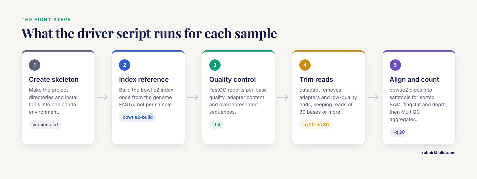
Now that each step works, record the whole sequence once. Create run_all.sh:

#!/usr/bin/env bash
set -euo pipefail

mkdir -p results/qc results/trim results/align results/counts logs

for r1 in data/fastq/*_R1.fastq.gz
do
  sample=$(basename "$r1" _R1.fastq.gz)
  r2="data/fastq/${sample}_R2.fastq.gz"

  echo "Processing ${sample}"

  fastqc -t 4 -o results/qc "$r1" "$r2"

  cutadapt -a CTGTCTCTTATACACATCT -A CTGTCTCTTATACACATCT \
    -q 20 -m 30 -j 4 \
    -o "results/trim/${sample}_R1.trim.fastq.gz" \
    -p "results/trim/${sample}_R2.trim.fastq.gz" \
    "$r1" "$r2" > "logs/${sample}.cutadapt.txt" 2>&1

  bowtie2 -x reference/genome \
    -1 "results/trim/${sample}_R1.trim.fastq.gz" \
    -2 "results/trim/${sample}_R2.trim.fastq.gz" \
    -p 4 2> "logs/${sample}.bowtie2.txt" | \
  samtools view -b -q 20 | \
  samtools sort -@ 4 -o "results/align/${sample}.sorted.bam" -

  samtools index "results/align/${sample}.sorted.bam"
  samtools flagstat "results/align/${sample}.sorted.bam" > "results/align/${sample}.flagstat.txt"
  samtools depth -a -q 20 "results/align/${sample}.sorted.bam" > "results/counts/${sample}.depth.txt"
done

multiqc results/ -o results/multiqc
echo "Done. See results/multiqc/multiqc_report.html"

Make it executable and run it:

chmod +x run_all.sh
./run_all.sh

Two lines of that script deserve explanation. set -euo pipefail makes the script stop on the first error, on any unset variable, and on any hidden failure inside a pipe, which converts silent corruption into a loud, immediate crash. The for loop derives the sample name from the read-1 file name, so adding sample C to the project means adding two files and rerunning one command, never editing the script.

The captured bowtie2 log (${sample}.bowtie2.txt) contains the aligner's own summary, including the overall alignment rate, which is the number to quote in a methods section.

From Shell Script to Workflow Engine

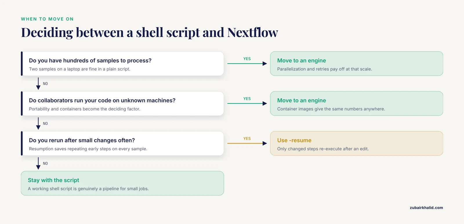
The shell script above is genuinely a pipeline, and for two samples on a laptop it may be all you need. Three pressures eventually push teams toward a dedicated workflow engine: hundreds of samples, heterogeneous computing resources, and collaborators who run your code on machines you have never seen.

Nextflow is the engine that much of the field converged on. Community pipelines built under the nf-core framework demonstrate the pattern at scale, with layered and modular architectures, multiple execution modes, and data-driven selection of methods at individual steps [1]. A Nextflow pipeline expresses each step as a process that declares its inputs, outputs, and the shell commands inside it, and the engine handles parallelization, retries, and resumption.

A minimal Nextflow translation of the FastQC step looks like this:

process FASTQC {
    tag "${sampleId}"

    input:
    tuple val(sampleId), path(reads)

    output:
    path "*_fastqc.html", emit: reports

    script:
    """
    fastqc -t ${task.cpus} ${reads}
    """
}

Running it looks like:

nextflow run main.nf -resume

The -resume flag is Nextflow's killer feature: rerunning after a change re-executes only the steps whose inputs or code changed. When you accidentally break something at step 5 of 9, you fix it and resume instead of repeating steps 1 through 4 on a hundred samples.

Containerization completes the portability story. A container image bundles a tool with its exact dependencies, so the same image produces the same numbers on your laptop, a university cluster, or the cloud. With a container-enabled profile, the engine runs every process inside its image. Research groups without infrastructure sometimes go further and assemble their own computing clusters for bioinformatics and biomedical work from the hardware up, which tells you how central reproducible execution has become to the field [5].

One honest caveat about architecture: domain-specific pipelines often contain steps with no clean one-sample-in, one-file-out structure. Group-level analyses, where samples are merged by condition and a control influences the result, resist naive modularization. An evaluation of agentic systems building a Nextflow DSL2 pipeline for CUT&Tag data found that all three systems produced pipelines with plausible documentation and file structure, yet none fully satisfied the requested analysis, and the most consequential shared failure was exactly this kind: each generated pipeline performed some form of group-level merging but failed to produce the requested merged-group reporting outputs, and sample-level MultiQC summaries disagreed with a hand-coded reference [6]. The lesson for hand-built pipelines is direct. Plan the group-level and reporting steps on paper before you write code for them, and test that the final reports contain what you promised.

How to Check That Your Pipeline Is Right

A pipeline that runs without errors tells you nothing about correctness. Build verification into the template:

1. Smoke test with tiny data. Keep two miniature FASTQ files (a few thousand reads) in test_data/. Every time you change the pipeline, run it on those files first. A full run that takes minutes rather than hours makes testing habitual.
2. Assert on outputs, not on absence of errors. After alignment, check that the mapped fraction in each flagstat file exceeds a floor you consider acceptable for your assay, and that every sample has a nonempty depth file. A five-line checking script that prints PASS or FAIL per sample is worth more than an hour of manual clicking.
3. Check one sample end to end by hand. Open the trimmed FASTQ, view a few aligned reads at a known locus, and confirm the biology and the files agree. Automation hides errors spectacularly well.
4. Separate validation data from training data. This principle extends beyond sequence data. A reproducible supervised classification pipeline for pathology reports improved performance precisely by constructing an in-domain holdout set matched to production data, facility-stratified sampling, and a blinded manual audit that revealed substantial label noise concentrated in rare categories, with estimated positive prevalence shifting from 0.500 to 0.398 on audit of 600 reports. Whatever your downstream model or hypothesis test, hold data back and audit labels before trusting the headline numbers.
5. Watch for domain-specific validation gaps. In clinical metagenomics, reviews note that many AI-assisted classification methods report strong results on simulated datasets or mock communities rather than prospective clinical material, and that reference database bias remains a persistent confounder [7]. If your pipeline touches classification against reference databases, ask what your database contains and when it was built.

Choosing and Justifying Analysis Choices

The word "template" can mislead you into thinking pipeline construction is mechanical. The steps are mechanical, the choices inside them are scientific judgments, and the field's own literature documents how much those judgments vary.

Reviews of metagenomics pipelines emphasize that tool selection and pipeline design remain fragmented, with real tradeoffs between speed, sensitivity, and compute requirements, and that hybrid approaches combining long nanopore reads with short Illumina reads can recover complete biosynthetic gene clusters that neither technology alone recovers well [3]. In phylogenetics, the UnFATE project made its design judgment explicit: from a pool of candidate single-copy orthologous markers, the authors selected the smallest subset that still produced a robust phylogeny, balancing potential missing data against probe cost, and wrapped the whole procedure in a user-friendly script so other laboratories could apply it [8]. In Salmonella genomic epidemiology, reviews of whole-genome sequencing find that incorporating genomic detail into quantitative microbial risk assessment remains difficult, despite abundant sequencing data, because the analytical connection between genomes and risk models is genuinely underdeveloped [9].

When you write your own pipeline, record three things about every consequential choice:

1. What the parameter does. Not "quality trimming was performed" but "bases with Phred quality below 20 were removed from read ends using cutadapt with -q 20."
2. Why this value. A sentence is enough. "Q20 corresponds to a 1 percent per-base error rate, and the per-base quality plots fell below Q20 after position 140."
3. What alternative you rejected. This is the line reviewers and collaborators ask about first.

Where AI Coding Agents Fit, and Where They Do Not

Coding agents can now draft pipeline scaffolding quickly, and it is tempting to treat that as a substitute for understanding the steps. The evidence says otherwise, in both directions.

On the cautionary side, the comparative evaluation of three agentic systems on an identical detailed prompt for a CUT&Tag Nextflow pipeline found that polished documentation and file structure were not evidence of correctness. None of the three systems fully satisfied the requested analysis, shared failure modes appeared across systems, and among the three, Codex came closest to the hand-coded reference implementation [6]. Separately, the Zero2Repo benchmark asked coding agents to build complete repositories from a requirements document, an interface contract, and an empty workspace, with hidden acceptance tests and binary pass or fail rewards. Even on tasks drawn from repositories that frontier models have almost certainly seen during training, the strongest agent solved 10 of 11 tasks, and every failing submission still passed 90 to 99 percent of the hidden tests, meaning the failures were concentrated in the last, hardest details rather than the scaffolding.

Read those two results together and the practical policy emerges: agents are excellent at generating the boilerplate you would otherwise type, directory structures, boilerplate process blocks, README skeletons, and unreliable at the domain-specific tail, the exact reporting outputs and analysis semantics your science requires. Use agents to accelerate the former, and treat every generated line in the latter category as a draft to verify against a tiny dataset where you know the right answer.

A Learning Path That Actually Works

If you are at the start of the road and want to learn bioinformatics seriously, the template-first approach doubles as a curriculum. You learn by building something real, then filling each gap as it bites: shell scripting when the loop confuses you, genomics file formats when SAM flags confuse you, statistics when you interpret coverage.

Structured programs validate this order. The Bioinformatics Mentorship and Incubation Program in Kenya put participants through intensive training for the first six weeks of a four-month program, then assigned them mini-projects, tracked them through weekly code review sessions, and closed with a final presentation. Across five cohorts, participants went on to secure master's scholarships and jobs, and the authors attribute the outcome to structured mentorship built around project-based learning [10]. The ingredients are visible in the design: real projects, regular code review, and a deadline. A formal bioinformatics course gives you the theory layer, sequence alignment algorithms, statistical genetics, machine learning foundations, but you cement it by shipping a pipeline against real data. If you have neither a mentor nor a course, weekly code review can be approximated by publishing your repository and asking for critique in community forums, and the project deadline can be approximated by a dataset you have promised to someone.

Common Mistakes and Limitations

1. Modifying raw data. Never write output into data/fastq/. If a trimming step overwrites input, a failed run has silently destroyed your only copy. The template's read-only raw directory exists to make this mistake impossible.
2. No sample sheet. Renaming files by hand, or encoding sample identity in file names alone, guarantees a mixup the week your collaborator adds three samples with names like final_final2. One CSV file, one source of truth.
3. Unrecorded tool versions. Six months from now, a tool update changes a default parameter and your numbers move. The versions.txt file from Step 1 is your defense. Record it before the first real run, not after the mystery appears.
4. Hard-coded absolute paths. A script that only runs on your machine, under your username, is not a pipeline. All paths in the template are relative to the project root on purpose.
5. Testing on full-size data only. If your smoke test takes four hours, you will skip it. Keep tiny test files and run them after every change.
6. Assuming clean logs mean correct results. A pipeline can exit successfully while producing biologically wrong output, for example a wrong reference genome that still aligns reads at a plausible rate. The verification habits in the checking section, hand inspection of one sample and assertions on summary statistics, exist because exit codes are not evidence.
7. Skipping the report-planning step for group-level analyses. Merged-group outputs and final reports are where both hand-built and agent-generated pipelines most often fall short, as the CUT&Tag evaluation showed [6]. Sketch every final table and figure before writing the code that produces them.
8. Building alone. Pipelines reviewed by other eyes converge on correct and portable designs faster. Weekly review sessions are the mechanism the mentorship program used, and any analog, a colleague, a lab meeting, a public repository, captures most of the benefit [10].
9. Confusing environment management with reproducibility. Conda solves dependency installation. Reproducibility also requires pinned versions, recorded parameters, versioned code, and stable inputs. Containers plus a workflow engine plus a sample sheet get you most of the way there.
10. Individual results need expert review. No template replaces judgment about whether a specific sample, run, or dataset is trustworthy. Route suspicious outputs to someone who knows the assay.

Frequently Asked Questions

Do I need to know how to program before building a pipeline from scratch?

You need working shell basics (navigating directories, loops, redirection) and enough familiarity with one scripting language to read a script. You do not need software engineering depth. The template above can be your first real program, and each concept appears exactly where you need it.

Should I start with shell scripts or go straight to Nextflow?

Start with shell scripts. You will understand every command you later put into a workflow engine, and debugging a plain script teaches you what the engine automates. Move to Nextflow when parallelism, resumption, or portability start to hurt.

How much computing power does a simple pipeline need?

A two-sample bacterial genome pipeline runs comfortably on a laptop with 16 GB of RAM. Human-genome-scale projects want a server or cloud instance with tens of GB of RAM and many cores, which is why the template is designed to move to a workflow engine later rather than being rewritten.

Can AI coding agents write my pipeline for me?

They can draft scaffolding quickly, but evaluations show plausible-looking generated pipelines can miss required analysis outputs even when file structure looks correct. Use agents for boilerplate, verify every domain-specific step yourself on a tiny dataset with known answers.

What belongs in a bioinformatics pipeline template?

Five things: a machine-readable sample sheet, read-only raw data, code separated from data, one directory per intermediate result type with predictable file names, and a single driver entry point that regenerates everything from raw data alone.

How do I know my pipeline results are correct?

Run a smoke test on tiny data, assert on summary statistics such as mapped read fraction, manually inspect one sample end to end, and validate downstream conclusions on held-out data that you never used while building the pipeline.

How long does it take to become comfortable building pipelines?

With focused effort, weeks to build your first simple pipeline and months to build one you would trust with a publication. Programs built around project-based learning with weekly code review compress this timeline by catching your errors while they are still cheap.

When should I use an established community pipeline instead of building my own?

When a well-maintained pipeline for your exact assay exists and fits your data, use it and invest your energy in the science. Build from scratch when your assay, design, or reporting requirements genuinely differ, or when you need to understand the machinery deeply enough to modify it.

Sources

1. Abstract 863: Scratch: A highly modular pipeline for single-cell cancer research
2. STATegra: Multi-Omics Data Integration - A Conceptual Scheme With a Bioinformatics Pipeline
3. Bioinformatics pipelines for Metagenomics: A review of data processing and functional annotation approaches
4. MicroRNA bioinformatics in precision oncology: an integrated pipeline from NGS to AI-based target discovery
5. Building a Computer Cluster for Bioinformatics and Biomedical Research from Scratch to Production
6. From Prompt to Pipeline: A Comparative Evaluation of Large Language Model Coding Agents for Reproducible Bioinformatics Pipeline Construction
7. Artificial intelligence in clinical metagenomic pathogen detection: A critical review of pipeline integrations, challenges, and future directions.
8. UnFATE: A Comprehensive Probe Set and Bioinformatics Pipeline for Phylogeny Reconstruction and Multilocus Barcoding of Filamentous Ascomycetes (Ascomycota, Pezizomycotina)
9. Quantitative microbial risk assessment for Salmonella: Inclusion of whole genome sequencing and genomic epidemiological studies, and advances in the bioinformatics pipeline
10. A mentorship and incubation program using project-based learning to build a professional bioinformatics pipeline in Kenya