How to Choose the Right Protein Bioinformatics Tool
By Dr. Zubair Khalid, DVM, MS, PhD ·
The difference between two protein bioinformatics tools is rarely that one is "better" in general, it is that each one wins on a different combination of accuracy, speed, input type, and how well its assumptions match your protein. The rule of thumb for choosing: define the exact question you need answered, find at least one independent benchmark that tested candidate tools on data like yours, and prefer the tool whose strengths match your bottleneck, whether that bottleneck is accuracy, compute time, or your own skill level.
This guide walks through that rule in practice. It covers the best protein bioinformatics tools for beginners options across the major task families, the pros and cons of each family, worked scenarios, and the mistakes that waste the most time. The advice is grounded in published benchmarking studies, because tool marketing is not evidence and a benchmark on data unlike yours is not evidence either.
Why "Which Tool Is Best?" Is the Wrong First Question
A recurring finding in the bioinformatics literature is that no single method consistently outperforms all others. A 2025 study in NAR Genomics and Bioinformatics put this plainly while introducing nf-core/multiplesequencealign, a framework for comparing multiple sequence alignment tools on high-performance computing systems. The authors note that many core bioinformatics problems are computationally hard, so developers build heuristic solutions, and each heuristic wins under different conditions. Multiple sequence alignment, the process of arranging protein sequences to line up homologous residues, is a textbook example. It is an NP-hard problem, meaning no known algorithm finds the guaranteed best answer efficiently for large inputs, so every aligner makes trade-offs [1].
The same pattern repeats across the protein tool ecosystem. In structure prediction, a benchmark of 1,337 protein chains deposited in the Protein Data Bank between July 2022 and July 2024 found that AlphaFold2 achieved the highest median TM-score at 0.96 and the lowest median RMSD at 1.30 angstrom, while ESMFold (TM-score 0.95, RMSD 1.74 angstrom) and OmegaFold (TM-score 0.93, RMSD 1.98 angstrom) traded a modest amount of accuracy for runs that are 10 to 30 times faster. The authors concluded that the performance differences were negligible for many proteins, meaning the faster alignment-free predictors are sufficient for numerous applications [2].
So the honest answer to "which tool is best" is: best for which protein, which question, and which constraint. The rest of this article gives you a repeatable procedure for answering that.
The Five Questions That Decide Your Choice
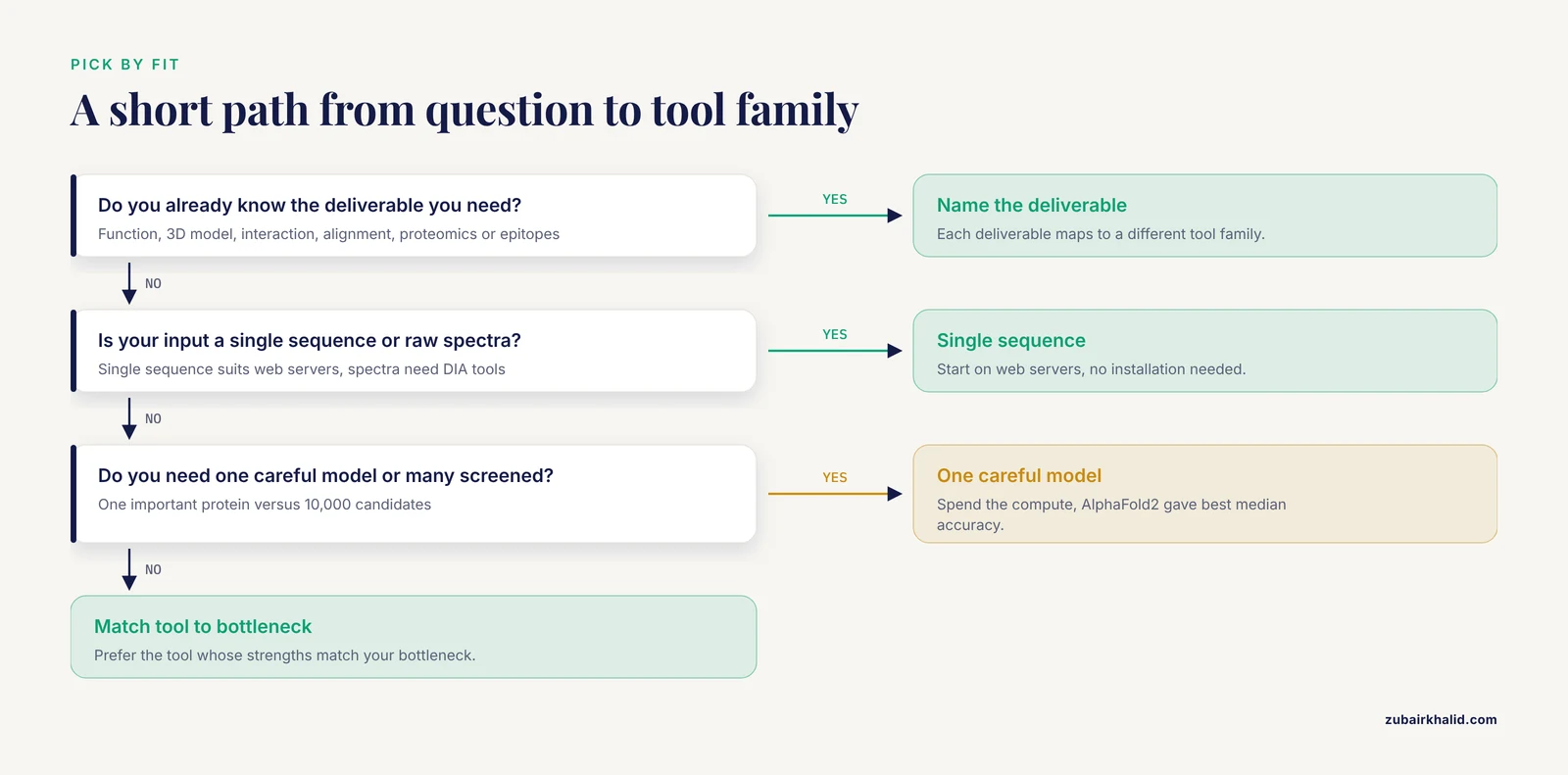
Before opening a single web server or installing anything, answer these five questions in writing. Beginners who skip this step almost always pick tools by popularity rather than fit.
1. What is the biological question and the deliverable?
"Do protein analysis" is not a question. These are questions with clear deliverables:
- I have a new protein sequence and want to know what it does (function prediction).
- I want a 3D model of my protein to interpret a mutation (structure prediction).
- I want to know whether two proteins interact and in what orientation (cofolding or docking).
- I want to align 500 homologous sequences to find conserved residues (multiple sequence alignment).
- I have mass spectrometry data and want quantified proteins (proteomics analysis).
- I want candidate B-cell or T-cell epitopes from an antigen for vaccine or diagnostic design (epitope prediction).
Each deliverable maps to a different tool family. A tool chosen before the question is defined will almost always be the wrong one.
2. What does your input look like?
A single sequence, a whole proteome, raw mass spectrometry spectra, or an existing set of homologs all demand different tools. ESMFold and OmegaFold accept a sequence directly and do not need to search for homologs, which is why they are called alignment-free. AlphaFold2 relies on multiple sequence alignments and, where available, structural templates, which is one reason it is slower but often more accurate on well-characterized families [2]. If your protein comes from an orphan family with few known relatives, the tools behave differently, and that difference should drive your choice.
3. What is your accuracy versus speed trade-off?
This is the trade-off beginners underestimate most. The Frontiers in Genetics benchmark quantified it directly: AlphaFold2 gave the best median accuracy, but alignment-free methods ran 10 to 30 times faster, and for many individual proteins the accuracy gap was negligible [2]. If you need one careful model of one important protein, spend the compute. If you need to screen 10,000 candidates, speed wins and modest accuracy loss per candidate may not matter for ranking.
The same logic appears in complex prediction. The LiPP benchmark set of 311 nonredundant lipid-protein complex structures evaluated AlphaFold 3, Chai-1, RoseTTAFold AA, DiffDock-L, and AutoDock Vina. AlphaFold 3 achieved the highest success rate at 76.1 percent under the RMSD below 2 angstrom criterion, but that success rate dropped to 47.2 percent for structures not seen during training. Meanwhile, physics-based docking with AutoDock Vina and some AI predictors largely preserved physical constraints, while other AI methods frequently violated them [3]. Two lessons follow. First, benchmark numbers from training-like data overstate what you will see on genuinely novel targets. Second, plausibility matters, a model with a good-looking score can still be physically impossible.
4. How will you validate the output?
Every prediction is a hypothesis. The Alpha&ESMhFolds database takes this seriously by storing paired AlphaFold2 and ESMFold models for the human reference proteome, mapping Pfam domains onto the 3D structures, and adding external quality metrics so users can select the better model for downstream analysis. One robust observation from that resource: regardless of overall model quality, both methods converge to high pLDDT values in regions covered by Pfam entries [4]. pLDDT is a per-residue confidence score from 0 to 100 produced by these structure predictors, and high values in known domain regions is exactly the kind of sanity check you should run on your own models.
5. Can you reproduce the run?
Reproducibility is a choice criterion, not an afterthought. Versioned workflow frameworks such as nf-core pipelines exist precisely because ad hoc tool runs cannot be reliably repeated or compared [1]. If you plan to publish, choose tools you can pin by version, run in a container, and describe in a methods section. If you are exploring, web servers are fine, but record the version and parameters anyway.
Side-by-Side Comparison of the Major Tool Families
The table below is the core of this guide. It maps protein bioinformatics tasks to representative tools, the kind of access beginners can expect, and the honest trade-offs. Details and citations for every row follow in later sections.
| Task | Representative tools | Access pattern | Main strengths | Main limitations |
|---|---|---|---|---|
| Multiple sequence alignment | Clustal-style aligners, tools deployable through nf-core/multiplesequencealign | Web servers for small jobs, command line for scale | Essential input for many downstream methods, mature ecosystem | NP-hard problem, no single aligner wins everywhere, results differ by dataset [1] |
| Structure prediction, single protein | AlphaFold2, ESMFold, OmegaFold | Web servers (ColabFold-style, ESMFold API), local GPU for AF2 | AF2 highest accuracy in benchmarks, ESMFold and OmegaFold 10 to 30 times faster [2] | Reduced accuracy for proteins lacking family annotations and for certain fold classes, speed-accuracy trade-off [2] |
| Comparing two structure predictors | Alpha&ESMhFolds | Web server and database | Paired AF2 and ESMFOLD human models with Pfam annotation and quality metrics [4] | Human proteome focus, still requires your own biological interpretation |
| Complex prediction and docking | AlphaFold 3, Chai-1, RoseTTAFold AA, DiffDock-L, AutoDock Vina | Web servers where available, local installation for docking | AF3 best success rate on lipid-protein benchmark, Vina physically grounded [3] | Performance drops sharply on unseen complexes, some AI methods violate physical constraints [3] |
| Protein function prediction | Blast2GO, PANNZER2, OrthoML2GO | Command line or web | Orthogroup-aware machine learning can outperform classic pipelines [5] | Distant homologs remain hard, annotation quality depends on database coverage [5] |
| Epitope and antigenicity prediction | IEDB analysis tools, BepiPred, ABCpred | Web servers | Free, well documented, widely used in published vaccine and diagnostic workflows [6] [7] | Predictions are screening tools, experimental validation is mandatory |
| Peptide property screening | ProtParam, ToxinPred, AllerTop, BIOPEP-UWM, Umami-MRNN | Web servers | Fast, beginner friendly, used in published food-peptide pipelines [8] | Narrow per-tool scope, you need a pipeline of several tools |
| Disorder and flexible linker prediction | CAID3-participating predictors | Web servers and standalone | Community critical assessment provides comparative performance data [9] | Different methods win in different scenarios, no universal winner [9] |
| Aggregation-prone region prediction | AmyloPick and established APR tools | Web or standalone | Rigorous statistical evaluation, interpretable four-feature model [10] | Predictive performance across the field remains limited, for example BAP reaches only 84 percent accuracy [10] |
| DIA mass spectrometry proteomics | DIA-NN, FragPipe, Spectronaut, DIA-Umpire, diaTracer | Command line, some GUIs | Quantified proteins and phosphopeptides from raw spectra, strong tool ecosystem [11] [12] | Tools differ in coverage and quantitative variation, workflow compatibility matters [11] [12] |
| Workflow orchestration and tool comparison | nf-core/multiplesequencealign, GEMsembler, Chaperone | Command line, HPC oriented | Standardized deployment, reproducibility, consensus building [1] [13] [14] | Steeper learning curve, designed for scale rather than one-off questions |
| Consensus model building | GEMsembler | Python package | Consensus models from multiple reconstruction tools can outperform any single model [13] | Specific to genome-scale metabolic models, needs multiple input models |
Tool Families Explained, With Pros and Cons
This section covers each family on its own terms. When you read pros and cons, keep question 3 from the previous section in mind: the con that disqualifies a tool for one project is irrelevant for another.
Multiple sequence alignment tools
An MSA is the backbone of comparative protein analysis. It feeds phylogenetics, conserved residue identification, domain boundary calls, and, historically, the homology searches inside structure predictors.
Pros. The MSA ecosystem is mature, with many free options and web servers suitable for a handful of sequences. Because MSAs feed so many downstream analyses, improving or standardizing them has outsized value.
Cons. Alignment is NP-hard, so every tool is a heuristic, and the nf-core framework authors emphasize that no single approach consistently outperforms all others. Their pilot framework integrates popular MSA tools and is designed to make rigorous, standardized performance evaluation routine, which tells you something important: even specialists no longer trust intuition alone when picking an aligner for a new dataset [1].
When to choose what. For fewer than a couple dozen sequences, any mainstream web-based aligner is fine and differences will rarely change your conclusions. For hundreds to thousands of sequences, or when you need a defensible, reproducible choice for publication, run more than one aligner through a standardized framework and report agreement. That is exactly the use case nf-core/multiplesequencealign was built for [1].
Protein structure prediction tools
This is the family beginners ask about most, and the one where benchmark data is most instructive.
AlphaFold2. The accuracy reference point. In the 1,337-chain benchmark it achieved a median TM-score of 0.96, a median GDT-TS of 94 percent, and a median RMSD of 1.30 angstrom [2]. TM-score and GDT-TS are global measures of how well a predicted structure overlays the experimental one, where values near 1.0 or near 100 percent indicate near-native models. RMSD, root mean square deviation, measures average atomic deviation in angstroms. AlphaFold2's approach uses multiple sequence alignments and templates, which helps accuracy on families with evolutionary information but costs runtime.
ESMFold and OmegaFold. These are alignment-free, language-model-based predictors. ESMFold reached a median TM-score of 0.95 and OmegaFold 0.93 in the same benchmark, both within practical striking distance of AlphaFold2 while running 10 to 30 times faster [2]. If you are screening many sequences, these are the rational default.
The same protein can differ between predictors. The Alpha&ESMhFolds resource exists because AlphaFold2 and ESMFold, built on different procedures, behave differently depending on the experimental information available for a protein. It stores paired models for the human proteome, updated after UniProt release 2025_04, adds Pfam domain annotations, and imports external quality metrics so you can pick the better model for your purpose [4]. For a beginner, the practical takeaway is that comparing two predictions of the same protein is one of the cheapest, most informative validation steps available.
Known weak spots. The Frontiers in Genetics benchmark found reduced accuracy across all three tools for proteins lacking family annotations, for leucine-rich repeat proteins, and for structures determined by NMR. Interestingly, alignment-free methods excelled at de novo designed proteins [2]. The authors even trained LightGBM classifiers on ProtBert embeddings and confidence metrics to predict when each method would fail, which is a glimpse of where the field is heading: choosing a predictor per protein, automatically.
Pros of the family overall. Free access, mature tooling, per-residue confidence scores like pLDDT that let you judge which parts of a model to trust.
Cons. Confidence scores are not accuracy guarantees, weak spots cluster in predictable but real protein classes, and models are static snapshots that may not represent alternative conformations.
Complex prediction and molecular docking
When your question involves two or more molecules, a protein and a lipid, a protein and a small molecule, or two proteins, you move from single-structure prediction to complex prediction or docking.
The LiPP benchmark is the clearest recent evidence on how differently these tools behave. Across 311 curated nonredundant lipid-protein complex structures, AlphaFold 3 led with a 76.1 percent success rate at the RMSD below 2 angstrom criterion, but fell to 47.2 percent on structures absent from its training data. Physics-based docking with AutoDock Vina and some AI predictors largely preserved intramolecular and intermolecular constraints, whereas DiffDock-L and RoseTTAFold AA frequently violated them [3]. In plain language: some methods produce answers that look right and are geometrically sensible, others produce answers that look right and are physically impossible, and only a benchmark tells you which is which.
Pros. Cofolding tools can get you a plausible complex model in minutes without parameters or receptor preparation. Docking tools like AutoDock Vina give you physically grounded poses and are decades old, well documented, and still used in current published pipelines [8].
Cons. Success rates on genuinely novel complexes are far lower than headline numbers suggest [3]. Treating any predicted pose as settled fact is the single most common beginner error in this family.
Protein function prediction
Given a sequence with no known function, homology-based annotation is the classic approach. The limitation, noted by the OrthoML2GO authors, is that distant homologs are hard to detect and annotate correctly, and sequencing growth keeps creating sequences that fall into that gap [5].
OrthoML2GO illustrates a modern pattern: layer machine learning on top of evolutionary information. It uses USEARCH for homology searches, orthogroup analysis based on OrthoDB version 12.0, and gradient boosting to refine Gene Ontology term assignments, applied in sequence after a k-nearest-neighbors step. Compared against Blast2GO and PANNZER2, it demonstrated improved prediction accuracy on test samples from humans, Arabidopsis, and a combined multi-taxon sample [5].
Pros. Web-accessible classics like Blast2GO remain approachable, and orthogroup-aware methods push accuracy further. Cons. Annotation transfers errors propagate silently, and confidence in a transferred function decays with evolutionary distance. For a beginner, treat predicted functions as ranked hypotheses and check them against domain architecture and literature.
Epitope prediction for vaccine and diagnostic design
Immunoinformatics pipelines are popular with beginners because the tools are web-based and the output feels concrete. Published work shows both the standard workflow and its ceiling.
A brucellosis diagnostic study used BepiPred, ABCpred, and the Immune Epitope Database analysis tools to predict B-cell epitopes from Brucella outer membrane proteins, then built two multiepitope fusion proteins and tested them experimentally. Fusion Protein 2 reached an AUC of 0.9849 with 93.90 percent sensitivity and 97.26 percent specificity in small ruminant sera, and an AUC of 0.9664 in bovine sera [6]. A Toxoplasma gondii study layered many tools to characterize Hsp90, a 708-residue, 81.93 kDa chaperone, predicting 50.85 percent alpha-helices and 15.68 percent beta-strands and nominating high-affinity MHC-binding epitopes such as the peptide SEDLPL [7].
Pros. Free web servers, clear step-by-step logic, and workflows you can copy from published papers. Cons. Every downstream claim depends on prediction quality, and epitope predictors produce long candidate lists that require prioritization. Notice that in both studies the computational step was followed by real experiments. That is the correct structure of the work.
Peptide screening pipelines
Food and bioactive peptide research offers the cleanest beginner-scale pipeline example. The tauco umami-peptide study moved from LC-MS/MS identification to screening against the BIOPEP-UWM database, prediction with Umami-MRNN, toxicity screening with ToxinPred, allergenicity screening with AllerTop, physicochemical profiling with ProtParam, and finally molecular docking of three selected peptides against the T1R1/T1R3 receptor with AutoDock Vina 1.2.7. Binding affinities ranged from -7.689 to -9.323 kcal/mol, with the peptide PDATGHTA strongest at -9.32 kcal/mol [8].
Pros. Each tool does one narrow job, the interfaces are simple, and the sequence of tools is a template you can adapt. Cons. You are chaining many weak predictors, and each step's assumptions compound. Docking scores, in particular, rank hypotheses rather than measure binding.
Intrinsically disordered region and linker prediction
Disordered flexible linkers connect folded domains and matter for construct design and fusion protein engineering. The CAID3 critical assessment evaluated nine such predictors, including seven that participated in the assessment, at residue, region, and protein levels, including on proteins sharing less than 30 percent sequence similarity with training sets. The result was a familiar one: different methods performed better in different scenarios, with several methods accurately identifying linker residues among other disordered residues and only a few performing well at the whole-protein level [9].
Pros. Community assessments like CAID give you comparative data instead of vendor claims. Cons. You must match the predictor to your scenario, which requires reading the evaluation, not the homepage.
Amyloid and aggregation prediction
Protein aggregation prediction remains genuinely hard. The AmyloPick authors report that a representative existing tool, BAP, achieves only 84 percent accuracy on hexapeptide classification [10]. Their contribution was an interpretable four-feature model that outperformed state-of-the-art methods on hexapeptides and performed comparably on aggregation-prone regions in full proteins, plus a statistical methodology for rigorous comparison [10]. The lesson for beginners generalizes: when a tool family reports accuracies in the mid-80s, plan for experimental follow-up on every candidate you care about.
Mass spectrometry proteomics tools
If your protein question involves measuring abundance, you enter the DIA, data-independent acquisition, ecosystem. Two recent evaluations are directly useful.
The phosphoproteomics evaluation compared DIA-NN versions 1.9.2 and 2.3, FragPipe, and Spectronaut across a human cell line and bacterial lysate, on both a 15-minute Orbitrap Astral gradient and a 90-minute Orbitrap Exploris gradient. Spectronaut provided the highest phosphoproteome coverage on the Astral workflow, while DIA-NN 1.9.2, DIA-NN 2.3, and FragPipe showed less quantitative variation. Library-free searches identified more phosphopeptides than spectral-library searches but produced different phosphopeptide profiles [11].
The label-free DIA comparison assembled four search workflows, DIA-NN, DIA-Umpire, diaTracer, and MSFragger-DIA, and four quantitation utilities, directLFQ, AlphaPeptStats, Triqler, and a simple t test, then scored every compatible combination on identifications, differential expression sensitivity, fold-change accuracy, and false discovery rate control using spike-in benchmark datasets. The study's practical output is a set of recommendations about which tool pairs work well together [12].
Pros. These are serious, actively developed tools with strong documentation. Cons. Your identifications and fold-changes depend on the tool and search strategy, so tool choice is a scientific decision, not an IT decision. Changing tools mid-project can change your results.
Orchestration frameworks and consensus methods
Three resources represent a step up in scale, and each earns a place here because it solves a problem beginners hit early.
nf-core/multiplesequencealign standardizes how MSA tools are deployed and compared on high-performance computing, so a performance claim becomes reproducible rather than anecdotal [1].
GEMsembler addresses a different consensus problem. Different automatic genome-scale metabolic model reconstruction tools produce models with different strengths for the same organism, so the authors built a Python package that compares cross-tool models, tracks the origin of each feature, and assembles consensus models from any subset. Consensus models built from four automatically reconstructed models of Lactiplantibacillus plantarum and Escherichia coli outperformed gold-standard manual models in auxotrophy and gene essentiality predictions [13]. The general principle travels beyond metabolism: when tools disagree, the disagreement itself is information.
Chaperone is a harness for computational protein design that integrates RFdiffusion3 with downstream tools including ProteinMPNN and AlphaFold 3, more than 50 tools in total. In an evaluation across nine design tasks it cut total token usage by 86 percent and GPU costs by 64 percent relative to baseline agents while increasing the design pass rate [14]. Its relevance to tool selection is simple: once your pipeline involves five or more tools, the bottleneck shifts from choosing each tool to making them work together reliably.
Comparing Tools on the Criteria That Actually Decide Choices
Criterion 1: Independent benchmark evidence on data like yours
The single strongest predictor of a good choice is a benchmark whose test data resembles your problem. Look for three features in any benchmark you consult. First, held-out data, meaning test proteins that could not have been in the training set. LiPP explicitly separated structures not seen during training and watched the success rate fall from 76.1 percent to 47.2 percent [3]. The CAID3 evaluation subset with less than 30 percent sequence similarity to training sets serves the same purpose [9]. Second, multiple metrics rather than one, because RMSD, TM-score, and GDT-TS can disagree [2]. Third, an honest failure analysis, like the finding that all three structure predictors struggle with leucine-rich repeats and proteins lacking family annotations [2].
A useful model of what rigorous comparison looks like at scale comes from outside the protein world: a nanopore signal segmentation study ran 5 tools across 16 datasets covering different kingdoms of life, segmented 160,000 reads, and scored results with an aggregate built from 12 metrics [15]. When you evaluate protein tools, that is the standard of thoroughness to look for in the literature, even if you will never run anything that large yourself.
Criterion 2: Match between tool assumptions and your data
Alignment-free predictors assume the language model has seen enough evolutionary signal in pretraining. Alignment-dependent predictors need homologs to exist in databases. Physics-based docking needs a credible binding site and reasonable parameters for your ligand. Cofolding tools perform best when something similar appeared in training. Ask, for each candidate tool, what it assumes about your input, and check whether your protein violates those assumptions.
A concrete example comes from evolutionary biology. A study of plastid outer envelope transporters in plants combined sequence-based analyses with structure-based tools specifically because the deep evolutionary distances involved made sequence alone insufficient. Structure-based comparisons uncovered recruitment events and homology that sequence methods missed, including a recent structural rearrangement in the protein OEP40 [16]. The tool choice followed from the data's properties, not from habit.
Criterion 3: Cost of being wrong
Ranking 10,000 peptides for a screening experiment tolerates a 16 percent error rate far better than designing a diagnostic antigen does. The brucellosis fusion protein study did not stop at epitope predictions, it expressed two fusion proteins and measured sensitivity and specificity against 198 small ruminant and 232 bovine serum samples [6]. Match your validation depth to the cost of being wrong.
Criterion 4: Your own capacity
Beginner capacity includes compute, command-line comfort, and time. Web servers minimize all three barriers and are the right entry point. Command-line tools and workflow managers pay off when jobs multiply or when reproducibility becomes mandatory. There is no virtue in running AlphaFold2 locally on a laptop-sized GPU when a web server answers your question, and no virtue in clicking through a web server 500 times when a script would take an afternoon.
Worked Scenarios
Scenario 1: You cloned a novel protein and want to know what it does
Start with function prediction. Run a homology search, then consider an annotation pipeline. If close homologs with known functions exist, classic tools like Blast2GO may suffice. If the sequence looks distant from anything well characterized, orthogroup-aware approaches such as OrthoML2GO were designed for exactly this gap and outperformed Blast2GO and PANNZER2 in head-to-head comparisons on human, Arabidopsis, and multi-taxon samples [5]. In parallel, predict the structure and check per-residue confidence. High pLDDT in regions that map to known Pfam domains is evidence the model is trustworthy in the places that matter for function [4]. Deliverable: a ranked list of candidate functions with supporting evidence, not a single confident claim.
Scenario 2: You need a 3D model to interpret a point mutation in a well-studied human protein
Your protein has abundant homologs and likely a human reference model already exists. Check Alpha&ESMhFolds first, because it stores paired AlphaFold2 and ESMFold models for the human proteome with Pfam annotations and quality metrics, and lets you select the better model [4]. If you must model a variant de novo and accuracy is the priority, AlphaFold2 delivered the best median accuracy in a recent benchmark [2]. If your mutation sits in a region with low confidence in both models, no tool will rescue that region, and the honest answer is that the model cannot adjudicate the variant there.
Scenario 3: You are screening a bacterial phosphoproteomics dataset for regulated sites
Your bottleneck is throughput and your tool family is DIA proteomics. The evaluation covering DIA-NN, FragPipe, and Spectronaut found that a 15-minute Orbitrap Astral gradient identified similar phosphopeptide numbers to a 90-minute Exploris gradient across all tools, that Spectronaut gave the highest coverage, and that DIA-NN versions and FragPipe gave less quantitative variation [11]. Choose based on which matters more for your study, maximal coverage or quantitative stability, and keep your search strategy, library-based or library-free, consistent because the two produce different profiles [11]. If you also need differential expression, consult the workflow compatibility findings from the label-free DIA comparison before pairing a search tool with a quantitation utility [12].
Scenario 4: You want to design a peptide and check it is not toxic or allergenic before ordering it
Follow the published peptide pipeline pattern: identify or propose candidate peptides, screen against a curated database such as BIOPEP-UWM, apply activity prediction, then filter with ToxinPred for toxicity and AllerTop for allergenicity, profile basic physicochemical properties with ProtParam, and only then, if a receptor structure is available, dock the survivors [8]. This ordering matters because cheap filters come first. Docking scores in the -7 to -9 kcal/mol range appear routinely in this literature and should be read as a ranking signal within your own candidate set, not as a predicted dissociation constant [8].
Scenario 5: Your pipeline now has six tools and your GPU bill is climbing
You have crossed into orchestration territory. Two published patterns apply. Use a workflow framework to standardize deployment and comparison, the way nf-core/multiplesequencealign does for aligners [1]. Or use a harness like Chaperone, which integrates RFdiffusion3 with ProteinMPNN, AlphaFold 3, and more than 50 other tools, and which reduced token usage by 86 percent and GPU costs by 64 percent while raising the design pass rate across nine tasks [14]. The general lesson is that integration overhead becomes the dominant cost at scale, and it is worth choosing tools that play well inside a managed workflow.
Common Mistakes and Limitations
Trusting benchmark numbers from training-like data. The drop from 76.1 percent to 47.2 percent success when AlphaFold 3 faced structures absent from its training data is the clearest recent warning [3]. Any evaluation that does not separate training and test data inflates performance, and the antimicrobial peptide prediction literature has been criticized on exactly this ground, with heterogeneous datasets and inconsistent protocols producing inflated estimates and potential data leakage [17]. Before trusting a tool's claimed accuracy, ask whether the evaluation held data out.
Reading a single metric as the whole story. TM-score, GDT-TS, RMSD, and pLDDT answer different questions and can disagree [2]. A model with an acceptable global RMSD can still misplace the one helix you care about. Check per-residue confidence, especially in the region your question concerns.
Comparing tools on different datasets and calling it a comparison. Much of the published performance literature suffers from inconsistent evaluation protocols. The AmyloPick authors built their contribution around statistical methodology that permits direct, rigorous comparison with other classifiers precisely because differing methodologies in the literature have prevented it [10]. When you compare two tools yourself, keep the input identical, pin the versions, and change one thing at a time.
Using a prediction as an endpoint. Every strong study in this space pairs prediction with experiment. The brucellosis epitope predictions became proteins that were expressed and tested against hundreds of serum samples [6]. The tauco peptide predictions became candidates selected for docking, one step in a longer chain [8]. A prediction that never meets data is a placeholder.
Chaining weak predictors and forgetting compounding error. The peptide pipeline in scenario 4 uses five or six tools in series. Each has its own error rate, and errors compound multiplicatively across steps. Design your pipeline so the cheapest, most reliable filters run first, and keep the number of stages small.
Ignoring the possibility that two tools disagreeing is the result. GEMsembler's central insight is that cross-tool disagreement identifies uncertainty worth resolving, and that combining models can outperform any single model [13]. If your two structure predictions disagree about a loop, that is a finding, not a nuisance.
Choosing a tool because it is popular or new. Popularity tracks visibility, not fit. The CAID3 assessment found that different disordered-linker predictors win in different scenarios [9]. The Frontiers benchmark found that the newest, flashiest option is not automatically the right one for your protein class [2]. Fit beats fashion.
A note on limits. No computational prediction replaces measurement, and individual research questions need domain expertise appropriate to the system. Use these tools to generate and prioritize hypotheses, then test them.
How to Build the Skills: A Practical Learning Path
For readers who want to learn bioinformatics rather than just borrow its tools, the path is shorter than it looks, because modern protein tools are unusually beginner-accessible.
Start with sequence questions on web servers. Homology searching, multiple alignment, and simple property calculations require no installation. The peptide property tools used in published pipelines, ProtParam for physicochemical profiles or ToxinPred for toxicity screening, run on plain sequences in seconds [8]. This teaches the core skill, framing a question a tool can answer, without any setup friction.
Move to structure web servers. Submit a sequence to a structure predictor, download the model, and inspect pLDDT alongside known domain annotations. Comparing AlphaFold2 and ESMFold outputs for the same protein teaches both the biology and the meta-lesson that tools disagree and disagreement is informative [4].
Learn one command-line workflow manager. nf-core pipelines are the community standard for reproducible, versioned bioinformatics at scale [1]. Running a published nf-core pipeline teaches containers, configuration, and reproducibility in one stroke. A structured bioinformatics course that covers the command line, a workflow manager, and interpretation of benchmark results will pay for itself quickly, but self-teaching through published workflows works too.
Read benchmarks, not documentation, when choosing. Documentation tells you how to run a tool. Benchmarks tell you whether you should. The studies cited throughout this article, from the 1,337-chain structure benchmark [2] to the 311-complex LiPP set [3] to the CAID3 disorder assessment [9], are readable by beginners and each one ends with practical guidance on method selection.
Frequently Asked Questions
What are the best protein bioinformatics tools for beginners?
For a first project, start with web servers matched to your question, a mainstream multiple sequence alignment server, a function annotation pipeline such as Blast2GO, and a structure predictor with per-residue confidence scores. These cover the most common beginner questions, run without installation, and connect to the published workflows you can imitate.
How do I choose between AlphaFold2, ESMFold, and OmegaFold?
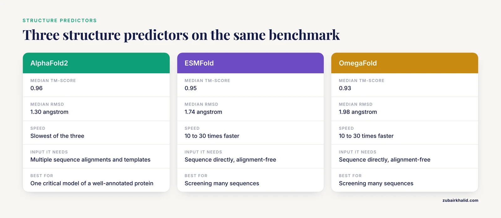
Choose by your accuracy-speed trade-off. AlphaFold2 gave the best median accuracy in a 1,337-chain benchmark, while ESMFold and OmegaFold run 10 to 30 times faster with only slightly lower accuracy, and for many proteins the difference is negligible. For screening many sequences, pick a fast alignment-free method, for one critical model of a well-annotated protein, spend the compute on AlphaFold2 [2].
Are predicted protein structures reliable enough to publish?
Regions with high pLDDT that overlap known Pfam domains are the most trustworthy parts of a model, and comparing independent predictions is a cheap sanity check. Low-confidence regions, proteins lacking family annotations, and certain fold classes are where predictions degrade, so scope your claims to the confident regions and validate experimentally where the stakes are high [4] [2].
Do I need to know how to code to use protein bioinformatics tools?
No, for single-sequence questions. Web servers handle alignment, annotation, structure prediction, and peptide screening without code. Coding becomes necessary when you process many sequences, need reproducibility for publication, or want to chain tools into a pipeline, at which point a workflow framework is the standard answer [1].
Why do different tools give different answers for the same protein?
Because most bioinformatics problems are computationally hard and every tool is a heuristic with different assumptions, so each wins under different conditions. Different predictors also draw on different information, for example alignment-dependent versus alignment-free structure prediction, and behave differently depending on what experimental data exists for your protein. Treat disagreement between two good tools as useful information about uncertainty rather than as a failure [4].
What is the fastest way to learn bioinformatics as a beginner?
Pick one small real question, such as annotating a protein you actually care about, and carry it through a full published pipeline, sequence search, alignment, structure prediction, and property screening. Then run one reproducible workflow framework pipeline to learn the command line. A structured bioinformatics course accelerates this, but a single complete end-to-end project teaches more than any amount of tool browsing.
Sources
- An nf-core framework for the systematic comparison of alternative modeling tools: the multiple sequence alignment case study.
- Balancing speed and precision in protein folding: a comparison of AlphaFold2, ESMFold, and OmegaFold.
- The LiPP Benchmark Set for Modeling Lipid-Protein Complexes: Comparison of Co-Folding and Docking Methods.
- Alpha&ESMhFolds: An Updated Web Server for the Comparison, Evaluation, and Annotation of Human AlphaFold2 and ESMFold Models.
- OrthoML2GO: homology-based protein function prediction using orthogroups and machine learning.
- Development and evaluation of multiepitope fusion proteins for serological diagnosis of animal brucellosis.
- Computational Prediction of Immunogenic Epitopes and Protein Structures of Heat Shock Protein 90 in Toxoplasma gondii.
- Identification and Virtual Screening of Umami Peptides in HPLC Fractions of Tauco by LC-MS/MS and Bioinformatics Tools.
- Comprehensive assessment of disordered linker predictions using data from the third critical assessment of protein intrinsic disorder.
- AmyloPick: A New Feature Selection Method and Proper Evaluation for Amyloid Hexapeptides and Aggregation-Prone Regions Prediction.
- Evaluation of Data-Independent Acquisition-Based Phosphoproteomics Analysis in Mammalian and Bacterial Systems.
- Comparison Study of Data Processing Workflows for Label-Free DIA Quantitative Proteomics.
- GEMsembler: consensus model assembly and structural comparison of genome-scale metabolic models across tools improve functional performance.
- Reliable and Efficient Agentic Protein Design with Toolset Harnessing.
- Dynamont: A comprehensive cross-species comparison of ONT segmentation tools.
- The evolutionary history of transporters of the plastid outer envelope of Chloroplastida- a structure-sequence comparison.
- Antimicrobial Peptide Databases and Prediction Tools: Toward a Standard Evaluation Framework.