Scaling Variant Calling to Thousands of Genomes in the Cloud

By Dr. Zubair Khalid, DVM, MS, PhD · 2026-11-11

By the end of this guide you will be able to take FASTQ files for hundreds or thousands of samples, lay them out as a batch, run a variant calling pipeline against them on AWS, estimate the bill before you launch, and validate the output against reference standards. You will also know the failure modes that turn a two-day run into a two-week one, and how to avoid each of them.

You need three things on hand before you start. First, an AWS account with permission to create S3 buckets and Batch compute environments (Google Cloud or Azure work equally well with the same design). Second, a workflow engine installed on a machine you control, such as Cromwell, Nextflow, or Snakemake. Third, your data in object storage: a reference genome bundle of roughly 10 GB and your sample FASTQ files. Everything else, containers, sample sheets, and pipeline code, is built step by step below.

Variant calling is the step that compares sequencing reads against a reference genome and reports the differences: single nucleotide variants (SNVs), insertions and deletions (indels), and structural variants (SVs). Batch variant calling in the cloud means processing many samples as one managed unit instead of one manual job at a time.

What Batch Variant Calling in the Cloud Means

Cloud bioinformatics rests on three properties that a single server cannot give you. Compute is elastic, so 500 samples can run as 500 parallel containers. Storage is an object store rather than a shared disk, so every task reads its inputs by URI. And the pipeline is defined as code, so the 2,000th sample is processed exactly like the first.

The scale is proven, not theoretical. The All of Us Research Program built Celeste, an open-source cloud architecture that has analyzed petabytes of participant genomic data and routinely handled fluctuating workloads of up to 9,000 whole-genome sequencing samples per month. Over 12 months of production inside a single AWS Region, Celeste coordinated around 200 million serverless function invocations and more than 20 million messages across 1.8 million bioinformatics, quality control, and clinical reporting jobs [1]. Two technologies carry that load: serverless orchestration (managed state machines and queues that trigger work without dedicated servers) and container orchestration (a system that schedules isolated software images onto compute capacity).

You do not need Celeste's engineering team to benefit from the same pattern. A workflow engine gives a small lab the same fan-out, retry, and provenance behavior, with the engine itself running on one small instance or even a laptop while the actual work runs in the cloud.

Architecture: Four Layers That Decide Whether You Scale

Layer 1: Object storage and data locality

Keep FASTQs, references, intermediates, and outputs in object storage (Amazon S3, Google Cloud Storage, or Azure Blob Storage). A quantitative comparison of distributed frameworks against conventional high-performance computing found that architectures where many compute nodes read and write through one network-attached shared filesystem stop scaling as nodes are added, while platforms that move compute to the data (data locality) remain efficient at biologically relevant sizes up to 100 gigabases of sequence [2]. The practical translation for a cloud batch: give each container a local scratch disk for BAM sorting and temporary files, and pass inputs and outputs as S3 URIs rather than mounting one giant network volume for the whole fleet.

Layer 2: Orchestration

Two orchestration patterns work at thousands-of-genomes scale. The first is serverless orchestration, the state machines and queues behind Celeste [1]. The second, and the one most labs adopt, is a workflow engine such as Cromwell, Nextflow, or Snakemake. The engine parses your pipeline definition, submits one containerized task per sample (the scatter), tracks every job, retries transient failures, and reassembles cohort-level outputs (the gather). Scatter and gather are the two halves of a batch: scatter means running the same per-sample tasks across all samples at once, gather means collecting their results into one downstream step.

Layer 3: Compute shape

Per-sample steps are independent, which makes them ideal for spot capacity (discounted cloud instances that the provider can reclaim at short notice), provided every task can retry from scratch on a fresh machine. Alignment and sorting are memory hungry. Variant calling is CPU hungry. The joint genotyping step, which combines all samples, needs dependable capacity because a spot reclaim in the middle of it wastes the most work.

Layer 4: Outputs and provenance

Write one small file per batch that records the reference build, container digests, engine version, and sample sheet checksum. Store it beside the results. Every downstream question about "which pipeline made this VCF" is then answerable from the data directory alone.

Choosing a Workflow Engine

Engine	Pipeline language	Common targets	Best fit
Cromwell	WDL	AWS Batch, Azure, Google Cloud, Terra	GATK-style germline pipelines, clinical reproducibility
Nextflow	Groovy-based DSL	AWS Batch, Azure, Google Cloud, HPC	Community pipeline collections, hybrid cloud and HPC estates
Snakemake	Python	Google Cloud, AWS, SLURM clusters	Python-centric teams, modular research pipelines
Swift/T	Swift	PBS Torque, SLURM, Cray, cloud	Very large fan-out batches across mixed infrastructure

WDL on Cromwell is the native language of GATK best-practice workflows and of Terra, the platform used to deploy containerized public-health workflows such as TheiaEuk, a species-agnostic fungal workflow that analyzed 752 Candida auris isolates from a southern Nevada outbreak [3]. Nextflow runs natively on AWS Batch and dominates community-maintained pipeline collections. Snakemake with Docker underpinned the CIMAC-CIDC clinical trial pipelines on Google Cloud, where benchmarking showed improved reproducibility, precision, and recall across validated truth sets [4]. Swift/T illustrates the design criteria that matter at production scale: transparent operation across PBS Torque, SLURM, Cray, and cloud environments, and formal criteria for robust, maintainable workflows that run on hundreds or thousands of samples at once [5]. Cromwell also runs on Azure, where it has driven PacBio HiFi long-read variant calling merged with clinical FHIR data in a single scalable pipeline [6].

Decide with three questions. Which cloud will you run on? Who will maintain the pipeline, and in which language are they fluent? Do you need a platform with a browser interface (Terra, DNAnexus) or a headless engine you drive from a terminal?

The Batch Format: Sample Sheets and Input Templates

Every engine consumes the same logical input: a table with one row per sample. The most portable batch variant calling cloud format is a plain TSV, because it survives Excel, version control, and every engine's converter. A minimal template:

sample_id	r1_fastq	r2_fastq	platform	library
sampleA	s3://acme-wgs-2026/fastq/sampleA_R1.fastq.gz	s3://acme-wgs-2026/fastq/sampleA_R2.fastq.gz	ILLUMINA	libA
sampleB	s3://acme-wgs-2026/fastq/sampleB_R1.fastq.gz	s3://acme-wgs-2026/fastq/sampleB_R2.fastq.gz	ILLUMINA	libB

Rules that prevent most batch failures before they happen:

Use stable sample IDs with letters, digits, underscores, dots, and hyphens only. Spaces break read groups and file names.
One row per library, not per sample, if a sample was sequenced across multiple lanes. The engine merges lanes.
Add an md5 column for each FASTQ if the files came from a sequencer vendor. A checksum mismatch caught at submission costs minutes, the same mismatch caught after alignment costs dollars.
Never edit the sheet between the pilot run and the full run. Regenerate it from the LIMS instead.

Validate the sheet with two commands before anything touches the cloud:

cut -f1 samples.tsv | tail -n +2 | sort | uniq -d
awk -F "\t" 'NR>1 {print NF}' samples.tsv | sort -u

The first command prints duplicate sample IDs, and empty output means none. The second prints the distinct column counts, and a single number means the file is rectangular.

The engine-facing template is a JSON file that maps workflow variables to values. Generate it from the sample sheet rather than by hand:

import csv, json

with open("samples.tsv") as handle:
    rows = list(csv.DictReader(handle, delimiter="\t"))

inputs = {
    "batch_variant_calling.sample_ids": [r["sample_id"] for r in rows],
    "batch_variant_calling.r1_fastqs":  [r["r1_fastq"] for r in rows],
    "batch_variant_calling.r2_fastqs":  [r["r2_fastq"] for r in rows],
}
json.dump(inputs, open("inputs.json", "w"), indent=2)

Running this on the two-row sheet above produces:

{
  "batch_variant_calling.sample_ids": ["sampleA", "sampleB"],
  "batch_variant_calling.r1_fastqs": [
    "s3://acme-wgs-2026/fastq/sampleA_R1.fastq.gz",
    "s3://acme-wgs-2026/fastq/sampleB_R1.fastq.gz"
  ],
  "batch_variant_calling.r2_fastqs": [
    "s3://acme-wgs-2026/fastq/sampleA_R2.fastq.gz",
    "s3://acme-wgs-2026/fastq/sampleB_R2.fastq.gz"
  ]
}

A Batch Variant Calling Cloud Example: 2,000 Genomes on AWS

This walkthrough runs a germline short-read pipeline (align, mark duplicates, call per-sample gVCFs, joint genotype) for a cohort of 2,000 genomes using Cromwell, WDL, and the AWS genomics stack. A gVCF is a per-sample file that records both variant positions and blocks of reference-matching genome, which is what joint genotyping consumes. The same structure works on Google Cloud or Azure with the backend configuration swapped.

Step 1: Create the bucket and credentials

aws configure

Expected output, using AWS's documented example values:

AWS Access Key ID [None]: AKIAIOSFODNN7EXAMPLE
AWS Secret Access Key [None]: wJalrXUtnFEMI/K7MDENG/bPxRfiCYEXAMPLEKEY
Default region name [None]: us-east-1
Default output format [None]: json

Then create one bucket and upload the FASTQs:

aws s3 mb s3://acme-wgs-2026
aws s3 sync ./fastq/ s3://acme-wgs-2026/fastq/

Expected output for each file:

upload: ./fastq/sampleA_R1.fastq.gz to s3://acme-wgs-2026/fastq/sampleA_R1.fastq.gz

Step 2: Build and upload the reference bundle

Download GRCh38 from NCBI RefSeq or your genome provider of choice, then build the index files on any Linux machine:

bwa index GRCh38.fa
samtools faidx GRCh38.fa
gatk CreateSequenceDictionary -R GRCh38.fa

Expected output from the aligner index step:

[bwa_index] Pack FASTA... 17.44 sec
[bwa_index] Construct BWT for the forward sequence... 498.02 sec
[bwa_index] Construct SA from BWT and Occ... 193.66 sec
[bwa_index] Construct BWT and Occ for the reverse sequence...
[bwa_index] Construct SA from BWT and Occ for the reverse sequence...

Timings vary with hardware. The command produces five index files (.amb, .ann, .bwt, .pac, .sa), the samtools faidx call produces GRCh38.fai, and the GATK call produces GRCh38.dict. The .fai and .dict must sit beside the FASTA, because GATK tools refuse to run without them. Also download the known-sites VCFs (dbSNP and the Mills indel set) that match your reference build, for base quality score recalibration, a recalibration step that corrects systematic per-base quality errors and belongs in every production run. Upload everything:

aws s3 sync ./reference/ s3://acme-wgs-2026/reference/GRCh38/

Step 3: Pin your container

Build one image that holds every tool the tasks need, then push it to Amazon ECR or your registry of choice and record the digest:

FROM broadinstitute/gatk:4.5.0.0
RUN apt-get update && apt-get install -y bwa samtools && apt-get clean

docker build -t wgs-tools:2026.01 .
docker tag wgs-tools:2026.01 registry.example.com/genomics/wgs-tools:2026.01
docker push registry.example.com/genomics/wgs-tools:2026.01

Pinning matters because a batch that spans days will outlive floating image tags. The digest recorded at build time is your proof that every sample ran the same binaries.

Step 4: Write the WDL tasks

Two tasks carry the per-sample work. The alignment task:

version 1.0

task align {
  input {
    String sample_id
    File reference_fasta
    File reference_index
    File r1_fastq
    File r2_fastq
    Int cpu = 8
  }

  command <<<
    set -euo pipefail
    bwa mem -t ~{cpu} -R "@RG\tID:~{sample_id}\tSM:~{sample_id}\tPL:ILLUMINA" \
      ~{reference_fasta} ~{r1_fastq} ~{r2_fastq} \
      | samtools sort -@ 4 -m 4G -o ~{sample_id}.sorted.bam
    samtools index ~{sample_id}.sorted.bam
  >>>

  runtime {
    docker: "registry.example.com/genomics/wgs-tools:2026.01"
    cpu: cpu
    memory: "32 GB"
  }

  output {
    File sorted_bam = "~{sample_id}.sorted.bam"
    File sorted_bai = "~{sample_id}.sorted.bam.bai"
  }
}

Parameters that matter here: -t sets aligner threads and should match the cpu runtime value, -R writes the read group (the metadata string that ties every alignment record to its sample), and samtools sort -m 4G caps memory per sorting thread so the container stays inside its limit.

The calling task:

task call_variants {
  input {
    String sample_id
    File reference_fasta
    File input_bam
    File input_bai
  }

  command <<<
    set -euo pipefail
    gatk MarkDuplicates -I ~{input_bam} -O ~{sample_id}.markdup.bam -M ~{sample_id}.dup_metrics.txt
    samtools index ~{sample_id}.markdup.bam
    gatk HaplotypeCaller -R ~{reference_fasta} -I ~{sample_id}.markdup.bam -O ~{sample_id}.g.vcf.gz -ERC GVCF
  >>>

  runtime {
    docker: "registry.example.com/genomics/wgs-tools:2026.01"
    cpu: 4
    memory: "32 GB"
  }

  output {
    File gvcf = "~{sample_id}.g.vcf.gz"
    File gvcf_tbi = "~{sample_id}.g.vcf.gz.tbi"
    File dup_metrics = "~{sample_id}.dup_metrics.txt"
  }
}

-ERC GVCF tells HaplotypeCaller to emit a gVCF instead of a plain VCF. Duplicate marking and sorting are the memory-hungry steps, which is why this task also carries 32 GB.

Step 5: Write the scatter workflow

workflow batch_variant_calling {
  input {
    Array[String] sample_ids
    Array[File] r1_fastqs
    Array[File] r2_fastqs
    File reference_fasta
    File reference_index
  }

  scatter (i in range(length(sample_ids))) {
    call align {
      input:
        sample_id = sample_ids[i],
        reference_fasta = reference_fasta,
        reference_index = reference_index,
        r1_fastq = r1_fastqs[i],
        r2_fastq = r2_fastqs[i]
    }
    call call_variants {
      input:
        sample_id = sample_ids[i],
        reference_fasta = reference_fasta,
        input_bam = align.sorted_bam,
        input_bai = align.sorted_bai
    }
  }

  output {
    Array[File] gvcfs = call_variants.gvcf
    Array[File] dup_metrics = call_variants.dup_metrics
  }
}

The scatter line is the entire batch mechanism: the engine instantiates both tasks once per element of sample_ids, up to whatever concurrency your backend allows, and the Array[File] output is gathered automatically.

Step 6: Generate inputs.json from the sample sheet

Run the Python converter from the previous section. Add the reference entries by hand once:

{
  "batch_variant_calling.reference_fasta": "s3://acme-wgs-2026/reference/GRCh38/GRCh38.fa",
  "batch_variant_calling.reference_index": "s3://acme-wgs-2026/reference/GRCh38/GRCh38.fa.bwt"
}

Step 7: Launch the batch

Configure Cromwell's AWS backend (a Batch job queue, a job definition, and S3 as the file system, per the Cromwell documentation), then:

java -Dconfig.file=application.conf -jar cromwell.jar run batch_variant_calling.wdl -i inputs.json

Expected output as the run progresses:

[info] Workflow 8bb9f4d4-6c1a-4f2e-9a3b-7d5c1e0f2a3b submitted.
[info] Workflow 8bb9f4d4-6c1a-4f2e-9a3b-7d5c1e0f2a3b finished: Succeeded.

The equivalent Nextflow launch, for teams using that engine, is:

nextflow run main.nf -profile awsbatch -params-file params.json -work-dir s3://acme-wgs-2026/work

Expected output:

N E X T F L O W  ~  version 24.x
Launching main.nf [focused_curie] DSL2 - revision: 5a1b2c3d4e

Step 8: Gather and joint genotype

For a handful of samples, combine the gVCFs directly:

gatk CombineGVCFs -R GRCh38.fa -V sampleA.g.vcf.gz -V sampleB.g.vcf.gz -O cohort.g.vcf.gz
gatk GenotypeGVCFs -R GRCh38.fa -V cohort.g.vcf.gz -O cohort.joint.vcf.gz

For 2,000 samples, do not combine everything in one process. Shard by interval instead: run GATK's GenomicsDBImport to ingest the per-sample gVCFs interval by interval, run GenotypeGVCFs per shard, then merge the shards:

bcftools concat -a -f shards.txt -Oz -o cohort.merged.vcf.gz
bcftools index -t cohort.merged.vcf.gz

Joint calling at cohort scale is well established. The 2,535-genome study discussed below used the Real Time Genomics population caller to genotype its whole cohort jointly on Amazon cloud infrastructure [7].

Step 9: Check the result, validate, and publish

Per-sample sanity checks first:

samtools flagstat sampleA.markdup.bam

Expected output (illustrative values):

620000000 + 0 in total (QC-passed reads + QC-failed reads)
607600000 + 0 mapped (98.00% : N/A)

Read the MarkDuplicates metrics file for each sample and flag outliers in percent duplication. Then check the cohort VCF:

bcftools stats cohort.joint.vcf.gz | grep "^SN"

Expected output:

SN	0	number of records:	4200000
SN	0	number of SNPs:	3900000

Finally, validate against truth. Run a Genome in a Bottle reference sample through the identical batch and compare:

hap.py truth.vcf.gz cohort.joint.vcf.gz -f highconf.bed -o giab_summary

The summary table has one row per variant type:

Type,TRUTH.TP,TRUTH.FN,QUERY.FP,METRIC.Recall,METRIC.Precision
SNP,...
INDEL,...

Recall is true positives divided by the sum of true positives and false negatives, and precision is true positives divided by the sum of true positives and false positives. Compare your numbers against the performance the same pipeline class achieves on the published truth sets, stratified by variant type. Publish with:

aws s3 sync s3://acme-wgs-2026/results/ ./results/

Then set lifecycle rules so work directories expire and only VCFs, gVCFs, CRAMs, QC reports, and the provenance file remain in long-term storage.

What the Run Costs

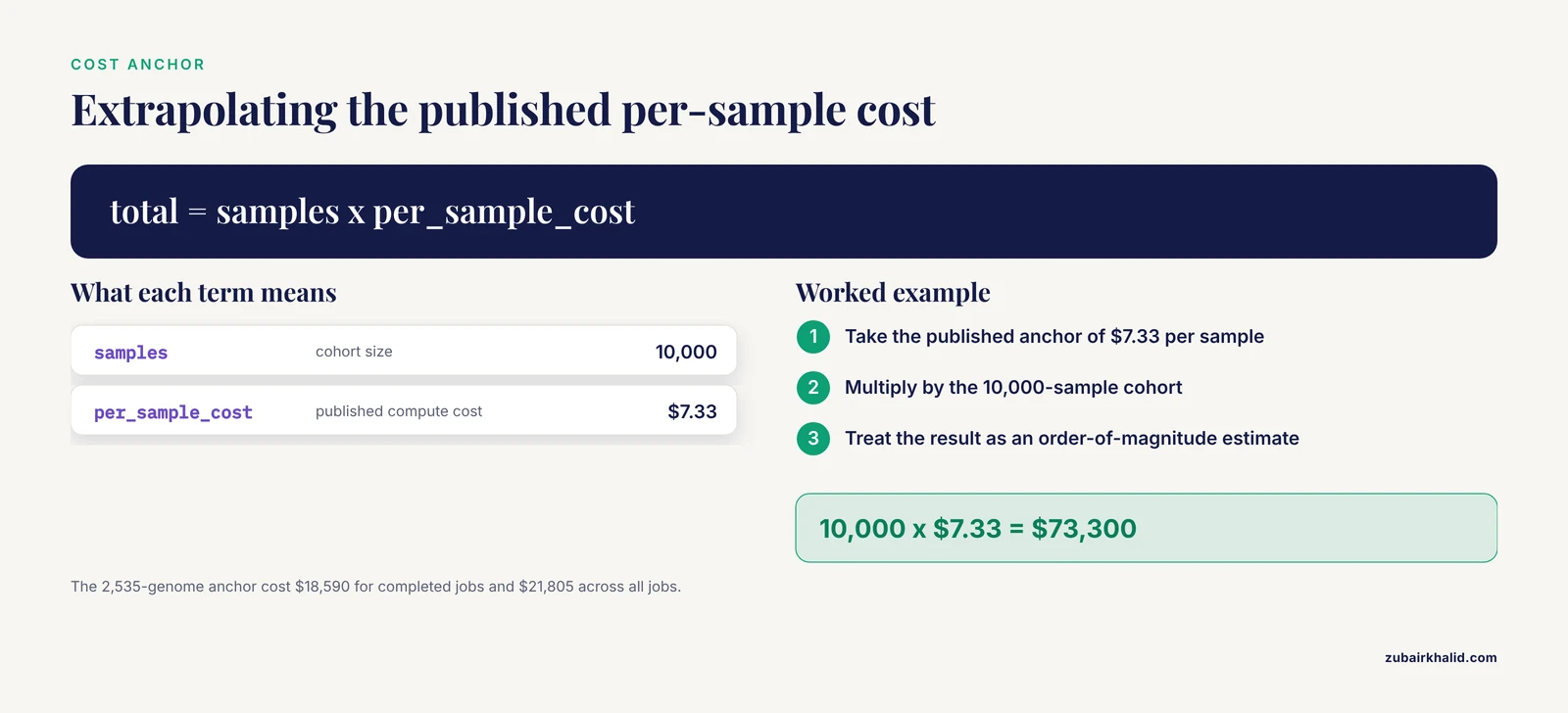
Worked calculation multiplying 10,000 samples by the published $7.33 per-sample compute cost to reach $73,300.

The clearest published anchor for batch variant calling in the cloud comes from a joint-calling run of 2,535 genomes from Phase 3 of the 1000 Genomes Project, executed on Amazon cloud infrastructure through the DNAnexus platform. The pipeline identified 68.3 million variants, finished in five days, and cost $7.33 per sample in compute, with totals of $18,590 for completed jobs and $21,805 across all jobs [7].

Published anchor (2,535 genomes, 2015 dollars):
  per-sample compute      $7.33
  completed-job total     $18,590
  all-jobs total          $21,805
  wall clock              5 days
  variants identified     68.3 million

Extrapolation at the same per-sample rate:
  10,000 samples x $7.33  =  $73,300

Read three lessons into those numbers. The gap between the completed-job and all-jobs totals is the price of failed and terminated work, so retries and a pilot batch are cost controls, not luxuries. The authors' analysis of cost dependence on data size suggested near-linear scalability, which is what makes the 10,000-sample extrapolation reasonable as an order-of-magnitude estimate [7]. And the anchor is dated: prices, instance families, and pipelines have all shifted since, so treat it as a sanity check and measure your own pilot bill before committing to a cohort-wide number. The other published anchor is the top of the range: population-scale programs processing petabytes on managed infrastructure [1], where engineering amortization, not per-sample compute, dominates.

Joint Calling and Case-Control Harmonization

If the batch feeds an association study, run every sample, cases and controls alike, through one pipeline version in one batch. A systematic investigation of false-positive inflation when using public controls such as gnomAD found that the inflated distribution of test statistics decreased substantially when the same variant caller and filtering pipelines were employed. Differences in library prep kits and sequencers did not affect the false-positive rate, and joint versus separate variant calling of cases and controls did not contribute to the inflation [8]. The operational conclusions are direct. Pipeline identity matters more than instrument identity, so harmonize the software before you worry about the sequencer. And you cannot repair a cohort that was processed in mismatched pipelines by joint calling it after the fact.

Long Reads at Scale

The same batch architecture carries long-read data with the tasks swapped. In an All of Us technical pilot comparing short-read and long-read sequencing, PacBio HiFi reads produced the most accurate results for both small and large variants in medically relevant genes, and the authors present a cloud-based pipeline that optimizes SNV, indel, and SV calling at scale for long reads [9]. On the orchestration side, Cromwell on Azure has been used to run PacBio HiFi variant calling and merge the results with FHIR clinical records and cloud-hosted Jupyter analysis in one pipeline [6]. Your sample sheet, scatter pattern, and provenance file stay exactly as they were. Only the align and call tasks change.

Validation, Benchmarking, and Human Review

Validation is a batch job too. Reference samples from the Genome in a Bottle (GIAB) consortium, compared with tools such as hap.py, vcfeval, and vcflib, are the standard way to assess a germline caller, and performance is not uniform across genomic regions or variant types, so benchmark per region of interest and per variant class. Because those benchmarking methods depend on hardware and libraries, a cloud-based benchmarking workflow that is independent of the machine running it lets you re-assess performance continuously as the pipeline evolves [10]. The CIMAC-CIDC cancer immunotherapy pipelines took exactly this approach, benchmarking Snakemake and Docker workflows across validated truth sets for precision and recall before clinical deployment [4].

Two review layers complete the picture. Structural variant calls benefit from human eyes, and SV-plaudit makes that scalable by generating one coverage image per SV, collecting reviewer verdicts through a web application, and emitting annotated VCF or tab-delimited reports. As a proof of principle, nine researchers evaluated 1,350 SVs each in a single hour [11]. Downstream, cloud-native specialty pipelines show the pattern extending past germline SNVs: Pgxtools analyzes sequence data for actionable variants in 13 pharmacogenes and was quality-verified against 1000 Genomes whole-genome data and CDC pharmacogenetics reference materials [12].

Common Mistakes and Limitations

Decision flow from a failed task through exit status 137, AccessDenied, NoSuchBucket and paired-read name errors to the matching fix.

Treating cloud storage as a shared disk. Architectures in which a growing fleet reads and writes through one network-attached filesystem degrade as nodes are added, a result demonstrated quantitatively for sequencing workloads [2]. Use object storage with per-task local scratch.

Mixing pipeline versions across a cohort. Association results inflate when cases and controls are processed differently, and the inflation tracks the pipeline, not the sequencer [8]. One batch, one version, recorded in the provenance file.

Trusting one genome-wide accuracy number. Caller performance varies by genomic region and variant type, so a single summary statistic can hide a collapsed recall in the regions you care about [10]. Stratify every benchmark.

Floating software and references. An unpinned container tag or an silently updated reference FASTA makes two batches incomparable. Pin digests, checksum the reference, and freeze both for the life of the project.

Underestimating the gather side. Per-sample scatter is the easy half. Joint genotyping over thousands of gVCFs is the step that needs sharding, dependable capacity, and the most planning.

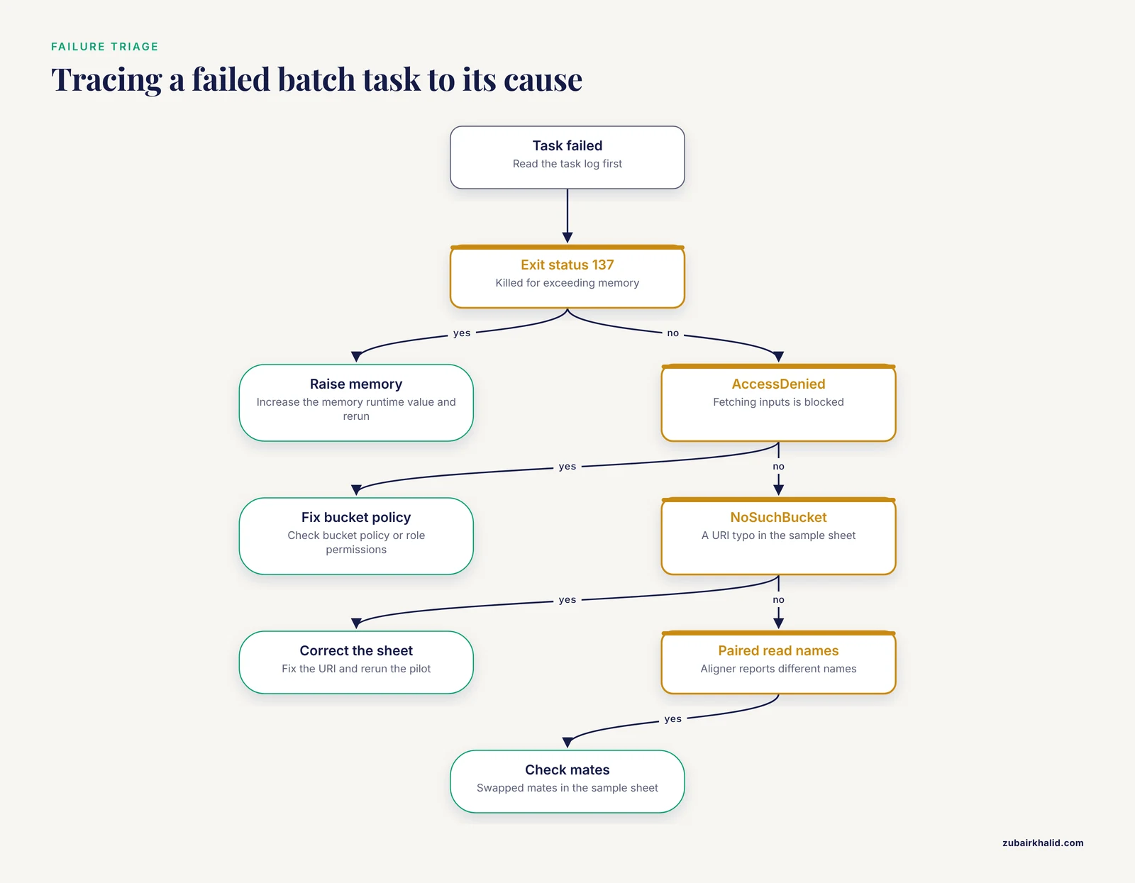
Ignoring sample sheet hygiene. Swapped mates surface deep in the run as the aligner error [mem_sam_pe] paired reads have different names, and duplicate IDs silently overwrite each other's outputs. Run the two validation commands from the format section on every sheet, every time.

Ignoring out-of-memory kills. A task that dies with Command exit status 137 was killed by the operating system for exceeding memory. Raise the memory runtime value and rerun, rather than retrying into the same wall.

Missing reference sidecars. GATK tools stop with an A USER ERROR has occurred message naming a missing .fai or .dict file. Rebuild the sidecars beside the FASTA and re-upload the whole prefix.

Credential and typo errors. Cromwell tasks that log AccessDenied when fetching inputs point at bucket policy or role problems, and NoSuchBucket means a URI typo in the sample sheet. Both are caught instantly by the 50-sample pilot.

Treating research output as clinical output. These pipelines produce research-grade calls. Any individual result used for clinical decision making requires appropriate laboratory accreditation, clinical-grade validation, and interpretation by qualified professionals, and published per-sample costs are historical anchors rather than quotes for your project.

Frequently Asked Questions

How many samples can a single batch run process?

There is no fixed cap, the ceiling comes from provider quotas, your scatter width, and your budget. Pilot with 50 to 100 samples, confirm the pipeline and the bill, then raise concurrency in steps while watching for API throttling.

Which workflow engine should I choose for cloud bioinformatics?

Choose the engine that matches your target platform and the skills of whoever maintains the pipeline. WDL on Cromwell fits GATK-centered germline work and Terra, Nextflow fits AWS Batch and community pipeline collections, and Snakemake fits Python-heavy teams.

Do I need joint calling if every sample already has a VCF?

Yes for cohort studies, because joint genotyping harmonizes genotype quality and allele frequency estimates across all samples at once. Per-sample VCFs suit some clinical workflows, but cohorts called in mismatched pipelines carry artifacts that joint calling cannot repair.

How do I validate a batch pipeline before trusting it on real data?

Run Genome in a Bottle reference samples through the identical pipeline and compare against their truth sets with hap.py or vcfeval, stratified by variant type and genomic region. A single genome-wide accuracy number hides regional problems.

Can the same batch architecture handle long-read data?

Yes, the sample sheet, scatter pattern, and provenance are unchanged. You swap the alignment and calling tasks for long-read tools, and published cloud pipelines already run PacBio HiFi calling at population scale this way.

What does batch variant calling in the cloud cost per genome?

Budget three components: per-sample compute, storage for intermediates and outputs, and the joint genotyping step. Published per-sample anchors exist, but prices and pipelines have shifted, so run a pilot, read the actual bill, and extrapolate linearly.

Which instance types should I use?

Memory-hungry steps such as alignment, sorting, and duplicate marking want memory-optimized instances, CPU-bound calling wants compute-optimized instances, and spot capacity suits per-sample tasks that retry cleanly. Keep joint genotyping on dependable capacity.

How do I stop the work directory from eating the budget?

Set lifecycle rules the day you create the bucket. Delete work directories on success, keep only VCFs, gVCFs, CRAMs, QC reports, and the provenance file, and archive or expire intermediates on a schedule.