Customizing Bar Plots for Genomic Feature Counts in Python
By Dr. Zubair Khalid, DVM, MS, PhD ·

By the end of this guide you will be able to take a table of genomic feature counts, for example gene counts per chromosome, counts of feature types from a GFF3 annotation, peak counts per ChIP-seq sample, or variant counts per functional class, and turn it into a publication-ready, fully customized bar plot in Python. You will learn how to load and aggregate the counts with pandas, draw a default bar chart with matplotlib, then systematically control ordering, color, labels, scales, error bars, faceting, and export settings. You will also see a grammar-of-graphics version using plotnine, and a checklist of mistakes that make genomic count plots misleading.
To follow along you need Python 3.9 or newer, the packages pandas, matplotlib, seaborn, and plotnine, and optionally Biopython plus the bcbio-gff parser if you want to read annotation files directly. Everything below runs in a Jupyter notebook or a plain script.
Why Bar Plots Work Well for Genomic Feature Counts
A genomic feature count is a non-negative integer attached to a discrete category. Examples include how many coding sequences sit on each chromosome, how many peaks each transcription factor contributes in a ChIP-seq experiment, or how many variants fall into each consequence class. When the question is "how much of each category is present," a bar plot answers it directly, because the length of each bar encodes the count and the category labels sit along an axis.
Visualization in biology has long struggled with the sheer size of high-throughput datasets, and reviewers have pointed out that the key challenge is helping readers benefit from large data volumes without being overwhelmed by them [1]. A well-made summary plot is one of the main defenses against that overload. Bar plots occupy a specific and useful niche in that toolbox: they summarize discrete tallies, while methods such as UMAP, PHATE, and related embeddings serve continuous or high-dimensional structure. A bar plot is the right tool when your data is genuinely categorical counts, and the wrong tool when you are trying to show relationships among thousands of individual entities.
Python has become the dominant language for this kind of work. The authors of plotnineSeqSuite note that bioinformaticians have been shifting toward Python and that providing R-style plotting interfaces in Python reduces the cost of switching languages [2]. The same trend drives the many domain-specific Python packages that now include their own visualization layers, from metabolic modeling frameworks to geospatial and structural biology tools [3], [4], [5]. Learning to customize a bar plot well is therefore a portable skill across almost every branch of python for bioinformatics.
Setting Up Your Environment
Install the core stack with pip:
python -m pip install --upgrade pip
python -m pip install pandas matplotlib seaborn plotnine biopython bcbio-gff
Check your versions so your results are reproducible:
import sys
import pandas as pd
import matplotlib
import matplotlib.pyplot as plt
import seaborn as sns
import plotnine as p9

print(sys.version)
print("pandas", pd.__version__)
print("matplotlib", matplotlib.__version__)
print("seaborn", sns.__version__)
print("plotnine", p9.__version__)
Expected output on a current install looks something like this, and the exact patch numbers do not matter as long as you record them:
3.11.5 (main, Sep  2023) [clang]
pandas 2.1.4
matplotlib 3.8.2
seaborn 0.13.2
plotnine 0.12.4
Recording versions matters because plotting libraries change default styles between major versions, and a figure that reproduces today may shift subtly after an upgrade.
A Bar Plot of Genomic Features in Python, Step by Step
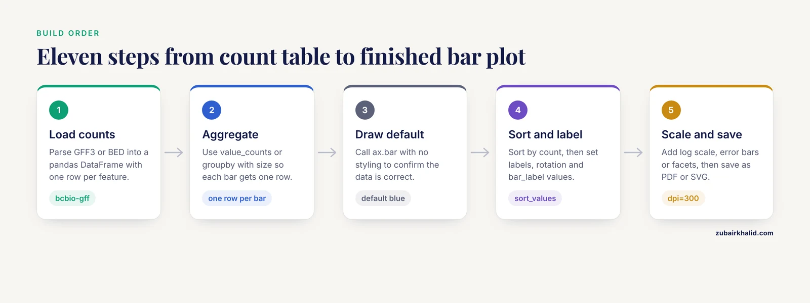
This walkthrough builds one plot through eleven small, verifiable steps. Each step adds one layer of customization, which is how you should approach real figures: change one thing, look at the result, move on.
Step 1: Get Feature Counts Into a pandas DataFrame
Most genomic pipelines end with a tabular file, a GFF3 or GTF annotation, a BED file of peaks, a tab-delimited count matrix, or a JSON summary. Python packages for biological data generally parse these formats into ordinary Python data structures so downstream code can treat them uniformly [6], and public repositories make the underlying data broadly available to any language [7]. For a GFF3 annotation you can use bcbio-gff, which plugs into Biopython:
from BCBio import GFF

rows = []
with open("genes.gff3") as handle:
    for record in GFF.parse(handle):
        for feature in record.features:
            rows.append({
                "chrom": record.id,
                "feature_type": feature.type,
            })

counts_df = pd.DataFrame(rows)
print(counts_df.head())
Expected output:
      chrom feature_type
0  chrI           gene
1  chrI           gene
2  chrI        mRNA
3  chrI        exon
4  chrI         CDS
If you do not have a GFF3 handy, create a synthetic DataFrame that behaves the same way. The rest of the walkthrough uses this synthetic data so every command is runnable:
import numpy as np
import pandas as pd

rng = np.random.default_rng(42)
chroms = [f"chr{i}" for i in range(1, 6)]
types = ["gene", "mRNA", "exon", "CDS", "pseudogene"]

counts_df = pd.DataFrame({
    "chrom": rng.choice(chroms, size=500, p=[0.3, 0.25, 0.2, 0.15, 0.1]),
    "feature_type": rng.choice(types, size=500, p=[0.4, 0.15, 0.2, 0.2, 0.05]),
})
print(counts_df["feature_type"].value_counts())
Expected output:
feature_type
gene          201
exon          103
CDS            98
mRNA           74
pseudogene     24
Name: count, dtype: int64
Your exact numbers will differ unless you use the same seed, but the shape of the output will match.
Step 2: Aggregate the Counts
Bar plots need one row per bar. Use value_counts for a single categorical variable, or groupby with size for combinations of variables:
type_counts = counts_df["feature_type"].value_counts().rename_axis("feature_type").reset_index(name="n")
print(type_counts)

chrom_type_counts = (
    counts_df
    .groupby(["chrom", "feature_type"])
    .size()
    .reset_index(name="n")
)
print(chrom_type_counts.head())
Expected output for the first table:
  feature_type    n
0         gene  201
1         exon  103
2          CDS   98
3         mRNA   74
4   pseudogene   24
Sanity check the aggregation before plotting. The counts column should sum to the number of input rows:
assert type_counts["n"].sum() == len(counts_df)If that assertion fails, you dropped rows during filtering or the category column contains NaN values, which value_counts excludes by default.
Step 3: Draw a Default Bar Plot
Start with the smallest matplotlib call that works, then customize it. This is the fastest way to confirm your data is correct before spending time on styling:
import matplotlib.pyplot as plt

fig, ax = plt.subplots(figsize=(6, 4))
ax.bar(type_counts["feature_type"], type_counts["n"])
ax.set_ylabel("Feature count")
ax.set_title("Genomic features by type")
fig.tight_layout()
plt.show()
You should see five bars in matplotlib's default blue, alphabetical category order on the x axis, and y axis ticks that matplotlib chose automatically. The default figure is correct but not finished. Everything after this step is customization.
Step 4: Sort Bars by Count Instead of Alphabetically
The most common complaint about default genomic bar plots is that pandas and matplotlib both order categories alphabetically, which buries the biological signal. Sort the DataFrame before plotting, because matplotlib draws bars in the order you pass them:
type_counts_sorted = type_counts.sort_values("n", ascending=False)

fig, ax = plt.subplots(figsize=(6, 4))
ax.bar(type_counts_sorted["feature_type"], type_counts_sorted["n"],
       color="#2C7FB8", edgecolor="black", linewidth=0.6)
ax.set_ylabel("Feature count")
ax.set_title("Genomic features by type (sorted)")
fig.tight_layout()
plt.show()
Now the tallest bar is at the left and the story of the data, that genes dominate and pseudogenes are rare, is visible before anyone reads a single number. When you instead want to preserve a biologically meaningful order, such as chromosome order chr1 through chrX, define the order explicitly with a categorical dtype:
chrom_order = ["chr1", "chr2", "chr3", "chr4", "chr5"]
counts_df["chrom"] = pd.Categorical(counts_df["chrom"], categories=chrom_order, ordered=True)
chrom_counts = counts_df["chrom"].value_counts().sort_index()
Step 5: Customize Labels, Typography, and Axis Behavior
Readable axes matter more than decorative color. Set explicit labels, rotate tick labels when category names are long, and control tick density:
fig, ax = plt.subplots(figsize=(6, 4))
bars = ax.bar(type_counts_sorted["feature_type"], type_counts_sorted["n"],
              color="#2C7FB8", edgecolor="black", linewidth=0.6)

ax.set_xlabel("Feature type", fontsize=12)
ax.set_ylabel("Number of features", fontsize=12)
ax.set_title("Genomic feature counts in the annotation", fontsize=13, pad=10)
ax.tick_params(axis="x", labelrotation=30, labelsize=11)
ax.tick_params(axis="y", labelsize=11)

for container in ax.containers:
    ax.bar_label(container, padding=3, fontsize=10)

ax.margins(y=0.08)  # headroom so count labels are not clipped
fig.tight_layout()
plt.show()
bar_label writes the exact count above each bar, which lets you drop gridlines and keep the plot clean. The ax.margins(y=0.08) call reserves 8 percent extra vertical space so those labels are not cut off at the top of the axes, a very common annoyance.
Step 6: Handle Wide Count Ranges With a Log Scale
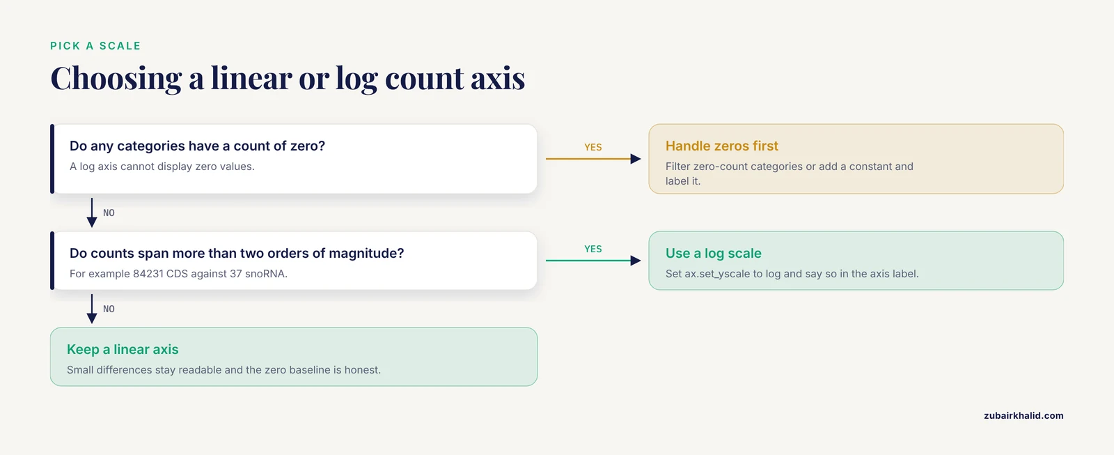
Genomic count data is usually skewed. A few feature classes have thousands of members and most have a handful, which makes small bars invisible on a linear axis. A logarithmic scale fixes the visibility problem, with one hard rule: log scales cannot represent zero, so filter or handle zero-count categories first.
skewed = pd.DataFrame({
    "category": ["CDS", "exon", "ncRNA", "repeat", "tRNA", "rRNA", "snoRNA"],
    "n": [84231, 79814, 12645, 987, 512, 148, 37],
})

fig, ax = plt.subplots(figsize=(7, 4))
ax.bar(skewed["category"], skewed["n"], color="#2C7FB8", edgecolor="black", linewidth=0.6)
ax.set_yscale("log")
ax.set_ylabel("Count (log scale)")
ax.set_title("Feature counts spanning four orders of magnitude")
for container in ax.containers:
    ax.bar_label(container, padding=3, fontsize=9)
fig.tight_layout()
plt.show()
On the log axis the 37 snoRNAs are now visible next to the 84,231 CDS entries. Always state in the axis label that the scale is logarithmic, because readers who miss it will misjudge the differences between bars by orders of magnitude.
Step 7: Grouped and Stacked Bars for Multi-Sample Comparisons
To compare feature counts across samples or conditions, reshape the data so each category is a row and each sample is a column, then choose grouped or stacked geometry. Grouped bars make within-category comparison easy, stacked bars make totals easy:
pivot = chrom_type_counts.pivot(index="chrom", columns="feature_type", values="n").fillna(0)

# Grouped bars
ax = pivot.plot.bar(figsize=(8, 4), width=0.8, edgecolor="black", linewidth=0.5)
ax.set_ylabel("Feature count")
ax.set_xlabel("")
ax.legend(title="Feature type", bbox_to_anchor=(1.02, 1), loc="upper left")
fig = ax.get_figure()
fig.tight_layout()
plt.show()

# Stacked bars
ax = pivot.plot.bar(figsize=(8, 4), stacked=True, edgecolor="black", linewidth=0.5)
ax.set_ylabel("Feature count")
ax.set_xlabel("")
fig = ax.get_figure()
fig.tight_layout()
plt.show()
Use stacked bars when the total per chromosome is the message. Use grouped bars when the comparison between feature types within each chromosome is the message. When a comparison spans more than two or three conditions, facet instead of stacking, which keeps each panel honest.
Step 8: Horizontal Bars for Long Feature Labels
Genomic category names get long, Gene Ontology terms, pathway names, pfam domains. Rotating long labels 45 degrees is a workaround that hurts readability. A horizontal bar plot keeps the labels intact:
go_terms = pd.DataFrame({
    "term": [
        "DNA-templated transcription",
        "[signal transduction](/knowledge/molecular-biology/signal-transduction)",
        "protein phosphorylation",
        "vesicle-mediated transport",
        "[chromatin remodeling](/knowledge/molecular-biology/chromatin-remodeling)",
    ],
    "n": [412, 318, 274, 190, 88],
}).sort_values("n")

fig, ax = plt.subplots(figsize=(7, 4))
ax.barh(go_terms["term"], go_terms["n"], color="#2C7FB8", edgecolor="black", linewidth=0.6)
ax.set_xlabel("Number of annotated genes")
for container in ax.containers:
    ax.bar_label(container, padding=3, fontsize=10)
fig.tight_layout()
plt.show()
Note the two adjustments that horizontal bars require. Sort ascending, because barh draws from the bottom up, so the largest bar should be last. Put the count axis label on the x axis rather than the y axis.
Step 9: Add Error Bars for Replicate Counts
If your counts come from biological replicates, for example peaks called independently in three samples, show the spread. Compute a summary per category and pass the interval to yerr:
replicates = pd.DataFrame({
    "feature_type": ["promoter", "enhancer", "insulator", "silencer"] * 3,
    "sample": ["rep1", "rep1", "rep1", "rep1",
               "rep2", "rep2", "rep2", "rep2",
               "rep3", "rep3", "rep3", "rep3"],
    "n": [120, 340, 45, 12, 128, 322, 51, 15, 117, 351, 48, 10],
})

summary = replicates.groupby("feature_type")["n"].agg(["mean", "std"]).reset_index()

fig, ax = plt.subplots(figsize=(6, 4))
ax.bar(summary["feature_type"], summary["mean"],
       yerr=summary["std"], capsize=4,
       color="#2C7FB8", edgecolor="black", linewidth=0.6,
       error_kw={"elinewidth": 1})
ax.set_ylabel("Mean count across replicates")
fig.tight_layout()
plt.show()
Say in the caption whether the bars show the mean and the whiskers show the standard deviation, the standard error, or a confidence interval, because readers cannot tell from the figure alone.
Step 10: A Grammar-of-Graphics Version With plotnine
plotnine brings ggplot2-style declarative plotting to Python, and its success in biological visualization is visible in packages such as plotnineSeqSuite, which builds sequence logos, alignment diagrams, and sequence histograms on top of it [2]. If you move between R and Python, the grammar keeps your mental model consistent. The same sorted bar plot looks like this:
import plotnine as p9

plot = (
    p9.ggplot(type_counts, p9.aes(x="reorder("feature_type", "n")", y="n"))
    + p9.geom_bar(stat="identity", fill="#2C7FB8", color="black", width=0.7)
    + p9.geom_text(p9.aes(label="n"), va="bottom", nudge_y=3, size=9)
    + p9.labs(x="Feature type", y="Number of features",
              title="Genomic feature counts")
    + p9.theme_classic()
    + p9.theme(axis_text_x=p9.element_text(rotation=30, ha="right"),
               figure_size=(6, 4))
)
plot.draw()
The key difference from matplotlib is that you never manually sort the plotting data. The reorder("feature_type", "n") expression inside aes tells the grammar to order the x axis by the y value. Faceting, which required manual figure management in matplotlib, is one function call: add + p9.facet_wrap("chrom") to split the plot by chromosome.
Step 11: Export for Publication
Journals and theses need specific formats and resolutions. Save vector output when you can, because it scales without losing quality:
fig, ax = plt.subplots(figsize=(6, 4))
ax.bar(type_counts_sorted["feature_type"], type_counts_sorted["n"],
       color="#2C7FB8", edgecolor="black", linewidth=0.6)
ax.set_ylabel("Number of features")

fig.savefig("feature_counts.pdf", bbox_inches="tight")   # vector, for LaTeX
fig.savefig("feature_counts.svg", bbox_inches="tight")   # vector, for Illustrator
fig.savefig("feature_counts.png", dpi=300, bbox_inches="tight")  # raster, for slides
dpi=300 is a safe default for print, and bbox_inches="tight" trims surrounding whitespace. Verify the exported file by reopening it, not by trusting the notebook preview, because label clipping sometimes only appears in the saved file.
Quick-Reference Table of Key Options
| Goal | matplotlib call | Notes |
|---|---|---|
| Sort bars by value | Sort the DataFrame with sort_values before plotting | matplotlib draws bars in data order |
| Bar fill and border | color, edgecolor, linewidth in ax.bar | Use one accent color for a single series |
| Count labels on bars | ax.bar_label(container, padding=3) | Add ax.margins(y=...) headroom |
| Log y axis | ax.set_yscale("log") | Zeros must be filtered or handled first |
| Horizontal bars | ax.barh | Sort ascending, label the x axis |
| Grouped or stacked | df.plot.bar(stacked=False or True) | Pivot long data to wide first |
| Error bars | yerr plus capsize in ax.bar | Define in the caption what whiskers show |
| Explicit category order | pd.Categorical(..., categories=..., ordered=True) | Use for chromosome order |
| Grammar-of-graphics | plotnine geom_bar(stat="identity") | reorder() sorts within aes |
| Facets | plotnine facet_wrap or seaborn catplot | One panel per condition or chromosome |
| Publication export | fig.savefig(..., dpi=300, bbox_inches="tight") | Prefer PDF or SVG for print |
Tips for Better Genomic Feature Bar Plots
Use one accent color for a single series. Color should encode information. When all bars come from the same variable, a single color is more honest than a rainbow, and reserving hue for a second variable, such as treatment group, keeps the encoding legible.
Choose colorblind-safe palettes. seaborn ships palettes designed for color-vision deficiency, and sns.color_palette("colorblind") is a drop-in replacement for defaults. Test your final figure by converting it to grayscale, since many readers will print it that way.
Normalize when totals differ. If samples have different total reads or different annotation sizes, raw counts confound biological signal with sequencing depth. Compute counts per million or another explicit normalization, and say in the axis label which one you used. Never mix raw and normalized counts in the same figure.
Build a style module and reuse it. Several established Python visualization frameworks emphasize standardized, publication-quality output through shared, modular design rather than one-off scripts [4]. You can get the same benefit cheaply by putting your figure defaults in one file:
# plot_style.py
import matplotlib.pyplot as plt

def set_genome_style():
    plt.rcParams.update({
        "font.size": 11,
        "axes.spines.top": False,
        "axes.spines.right": False,
        "figure.dpi": 110,
        "savefig.dpi": 300,
    })
Then every notebook starts with from plot_style import set_genome_style and your figures look consistent across a manuscript.
Treat plotting as part of the analysis loop, not a final decoration step. Interactive tools for single-cell data were built specifically because researchers iterate between programmatic analysis and visual exploration, and that loop is where insights actually appear [8]. Expect to redraw your bar plot several times as you refine the category definitions, the normalization, and the ordering.
Automate the boring parts. If you produce the same class of figure for every project, wrap the aggregation and plotting into one function that takes a DataFrame and a category column. Larger platforms in sequence analysis have moved in exactly this direction, automating feature extraction, model evaluation, and visualization behind a consistent interface [9], and the same principle scales down to a single plotting helper in your own repository.
Common Mistakes and Limitations
Alphabetical ordering hides the pattern. This is the single most frequent flaw in submitted figures. Every bar plot of genomic features in python should be sorted by value, by a biological ordering such as chromosome position, or explicitly justified as alphabetical.
Truncated y axes exaggerate differences. Count bars encode magnitude by length, so a y axis starting at a nonzero value visually inflates small differences. Keep the axis starting at zero for raw counts, and reserve non-zero baselines for plots of position or index, where the convention differs.
Log scales with zero counts crash or distort. ax.set_yscale("log") on data containing zeros produces masked or dropped bars and matplotlib warnings. Filter zero-count categories, or add a constant and label the transformation clearly, and never silently drop categories the reader should know about.
Overstuffed categories. A bar plot with 80 categories is unreadable. Collapse rare categories into an "other" bar, aggregate to a coarser level, or facet. If your real question involves structure or transitions among many entities rather than tallies, dimensionality-reduction methods such as UMAP, which was applied specifically to visualize single-cell data structure, are a better fit than any bar chart [10], and methods such as PHATE and SONG exist for data that mixes discrete clusters with continuous progressions [11], [12]. Match the visualization to the question.
Ignoring sequencing depth and annotation size. Two samples with different total mapped reads will differ in every raw count for reasons unrelated to biology. Aggregate counts should be normalized or at least reported alongside library sizes, and this applies to peak counts, variant counts, and feature counts alike.
Version drift in defaults. seaborn 0.13 changed several APIs, including how hue and palette interact, and passing a palette without a hue now triggers a FutureWarning and eventually an error. Pin your package versions in the project environment and record them with every figure.
Mutating the DataFrame you are plotting. Chained assignment triggers the pandas SettingWithCopyWarning and can silently fail. Assign new columns with .loc or assign on the DataFrame itself rather than through a slice.
Copying code without checking the result. The fix for every plotting bug is the same habit: print the DataFrame you are about to plot, confirm the row count and the column names, and confirm the axis labels match the columns you intended. A wrong column name is the most common cause of a plot that renders beautifully and answers the wrong question.
A final limitation applies to interpretation rather than code. Counts describe the annotation or the experiment that produced them, and a bar plot can only be as trustworthy as the pipeline upstream of it.
How to Check Your Plot Is Right
Verification is short and mechanical. Run these three checks after any customized bar plot:
- Sum check.
df["n"].sum()must equal the number of records you started with, or the difference must be explained by explicit filtering. - Spot check. Pick the tallest and shortest bars and confirm those values against the raw table with
df.nlargest(3, "n")anddf.nsmallest(3, "n"). - Axis check. Confirm the axis label states the unit and the scale, for example "counts per million" or "count (log scale)", and that zero-count categories were handled deliberately.
assert type_counts["n"].sum() == len(counts_df)
print(type_counts.nlargest(3, "n"))
print(type_counts.nsmallest(3, "n"))
These checks catch ordering errors, aggregation drops, and silent category loss, which together account for most incorrect count figures.
Where to Go Next
Once bar plots are routine, three directions extend the skill. For sequence-oriented work, plotnineSeqSuite provides ggplot2-style sequence logos, alignment diagrams, and sequence histograms in Python, which pairs naturally with the grammar you learned here [2]. For dynamical modeling of metabolic networks, MASSpy extends the COBRApy ecosystem with simulation and visualization of kinetic models [3], and its figures follow the same customization principles. For sequence-design evaluation, the seqme library provides diagnostics and visualization functions alongside its metrics [13], and a foundation in Python, Biopython, and pandas from any standard biopython tutorial carries directly into all of these tools.
Frequently Asked Questions
Which Python library should I use for bar plots of genomic feature counts?
Use matplotlib when you need fine-grained control over every element, seaborn when you want statistical summaries and palettes with less code, and plotnine when you prefer ggplot2-style declarative syntax or move between R and Python. All three render through the same underlying figure model, so the choice is about workflow, not capability.
How do I install the packages I need?
Run pip install pandas matplotlib seaborn plotnine biopython bcbio-gff in your environment. If you use conda, install from the conda-forge channel instead, and record the versions you installed so figures remain reproducible.
How do I plot counts directly from a GFF3 or BED file?
Parse the file into a pandas DataFrame first, then aggregate with value_counts or groupby. bcbio-gff reads GFF3 and GTF through Biopython's feature model, and BED files load with pd.read_csv(sep="\t", header=None) followed by column naming.
How do I sort bars by count instead of alphabetically?
Sort the DataFrame with sort_values("n", ascending=False) before calling ax.bar, because matplotlib draws bars in data order. In plotnine, wrap the x aesthetic in reorder() instead of touching the data.
When should I use a log scale on a count bar plot?
Use it when your counts span more than about two orders of magnitude, and only after handling zero-count categories, which a log axis cannot display. Label the axis so readers know the scale is logarithmic.
How do I add error bars for replicate counts?
Aggregate replicates per category with groupby().agg(["mean", "std"]), then pass the standard deviation or interval to the yerr argument of ax.bar with capsize for the whisker caps. State in the caption what the bars and whiskers represent.
How do I export my bar plot for publication?
Call fig.savefig with the target format, dpi=300 for raster files, and bbox_inches="tight". Prefer PDF or SVG for journals because vector output scales without quality loss, and always reopen the saved file to check for clipped labels.
Can I make ggplot2-style bar plots in Python?
Yes. plotnine implements the ggplot2 grammar in Python, and biological packages such as plotnineSeqSuite build directly on it to provide R-like visualization APIs for sequence data. The syntax differs from matplotlib but the customization concepts, ordering, color, labels, and facets, transfer directly.
Sources
- Visualizing biological data-now and in the future
- plotnineSeqSuite: a Python package for visualizing sequence data using ggplot2 style
- MASSpy: Building, simulating, and visualizing dynamic biological models in Python using mass action kinetics
- GeospaceLAB: Python package for managing and visualizing data in space physics
- detritalPy: A Python-based toolset for visualizing and analysing detrital geo-thermochronologic data
- A fast and efficient python library for interfacing with the Biological Magnetic Resonance Data Bank
- RCSB Protein Data Bank: Celebrating 50 years of the PDB with new tools for understanding and visualizing biological macromolecules in 3D
- Sciviewer enables interactive visual interrogation of single-cell RNA-Seq data from the Python programming environment
- SeqHIVE: a Python package to convert the biological sequences to informative vectors for sequence property predictions
- Dimensionality reduction for visualizing single-cell data using UMAP
- Visualizing Structure and Transitions in High-Dimensional Biological Data
- Dimensionality reduction for visualizing high-dimensional biological data
- seqme: a Python library for evaluating biological sequence design from generative models