Choosing the Right Background Set for Enrichment Analysis
By Dr. Zubair Khalid, DVM, MS, PhD ·

An enrichment analysis is only as honest as its denominator: a whole-genome background counts thousands of genes your RNA-seq experiment never measured, while an expressed-genes background counts only the genes your pipeline could actually detect. The rule of thumb for choosing the right background set for enrichment analysis in RNA-seq is simple. Use the genes your differential expression step actually tested, keep that background identical for every list you compare, and report its size next to your results.
This guide walks through the main background set options with their pros and cons, the criteria that settle real decisions, worked scenarios drawn from published RNA-seq studies, and a troubleshooting checklist for the failures that surface during peer review and reruns.
Why the Background Set Matters in RNA-seq Enrichment Analysis
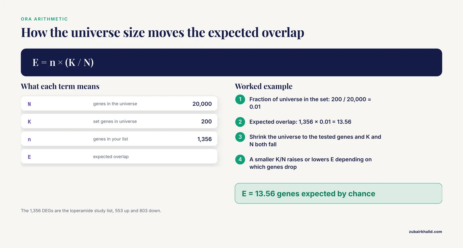
Enrichment analysis asks whether genes from a predefined set, such as a curated pathway, appear in your results more often than chance would predict. Two families of methods dominate RNA-seq work. Over-representation analysis (ORA) starts from a thresholded list of differentially expressed genes (DEGs) and tests each set with a hypergeometric or Fisher's exact test, which computes the probability of seeing an overlap this large if the list were drawn at random from a reference pool. Ranked-list methods such as GSEA (gene set enrichment analysis) instead use all measured genes ordered by a statistic and walk down the ranking to look for set concentrations at the extremes. Both families compare your genes against a reference pool, and that pool is the background set, also called the universe.
For ORA the dependence is explicit, because the test needs four numbers: the number of genes in the universe, the number of set genes in the universe, the number of genes in your list, and the number of set genes in your list. The expected overlap equals the list size multiplied by the fraction of universe genes that belong to the set. Change the universe and the expected overlap moves, sometimes enough to create or destroy a significant call.
RNA-seq makes this choice unusually consequential because detection is far from uniform. Poly(A) capture enriches messenger RNA by selecting polyadenylated transcripts, and it fails to capture non-poly(A) transcripts or partially degraded mRNAs, which also makes it incompatible with RNA from formalin-fixed paraffin-embedded (FFPE) samples. Ribosomal RNA depletion retains a broader transcript space and works on degraded material [1]. On top of library preparation, nearly every pipeline filters low-count genes before testing. The set of genes that could ever reach your DEG table is therefore much smaller than the annotation, and a background that ignores this mismatch answers a question about a genome your data never observed.
The distortions run in both directions. Inflating the universe with genes that could never enter your list shrinks the expected overlap for sets made of detectable genes, which makes those sets look more enriched than they are. Inflating it with genes that belong to a set but are silent in your tissue raises the expected overlap, which pushes that set toward non-significance. Both distortions come from the same mistake, a denominator that describes a different experiment than the one you ran. One of the most common RNA-seq errors in enrichment analysis is exactly this universe mismatch, and it is invisible in the output, because the software prints a p-value either way.
Ranked-list methods push the same decision into a different corner. GSEA takes no universe argument, so whatever enters the ranking silently becomes the background. That variant of the problem is covered under Option 6 below.
Background Set Options for RNA-seq Enrichment Analysis
Six options cover essentially every RNA-seq situation. Each has real pros and cons, and the right pick depends on your platform, your filtering, and the comparison you need to defend.
| Background option | What it contains | Best suited for | Pros | Cons | Typical failure mode |
|---|---|---|---|---|---|
| Whole genome or full annotation | Every gene in a reference annotation, about 20,000 protein-coding genes in human | Microarray-style data, quick exploratory scans | Simple, stable, no filtering decisions to defend | Counts genes your library prep cannot capture and your filters removed | Well-detected sets look spuriously enriched, tissue-silent sets get diluted |
| All quantified features | Every row of your count matrix | A base layer before filtering, quick checks | Reflects what the pipeline measured | Includes near-zero count noise | Noise features pad the denominator |
| Expressed genes after a filter | Genes passing a pre-specified rule, for example counts per million above 1 in at least 2 samples | Most bulk RNA-seq ORA | Matches detectability, standard, easy to report | Threshold choice changes the universe | Post hoc threshold tuning makes results flexible |
| Genes tested in the DE step | Results table rows with a valid p-value | The most defensible ORA default | Matches the null hypotheses actually tested | Needs plumbing into the tool | Silent truncation if the list is not a subset of the universe |
| Platform or protocol matched | Array probes, or detected genes rebuilt per protocol and cohort | Cross-platform, FFPE, and multi-cohort studies | Apples-to-apples comparisons | More bookkeeping, one universe per cohort | Carrying one cohort's universe into another |
| Full ranked list (GSEA family) | All quantified genes ranked by a statistic, no DEG cutoff | Graded, threshold-free evidence | Uses effect sizes, avoids arbitrary cutoffs | No explicit universe parameter, silent exclusions | Genes dropped before ranking are never tested |
The sections below explain each option on its own terms. A later section compares them on the criteria that actually settle arguments.
Option 1: Whole Genome or Full Annotation
This background is every gene in a reference annotation, roughly 20,000 protein-coding genes in the human genome, sometimes extended to non-coding genes. Many tools fall back on it when you do not supply a universe, either all genes in the annotation database or all genes appearing in the gene set file.
It is the right choice in two situations. Microarray-style data interrogate most genes by design, so the array's probe set approximates the genome and a full annotation background is a reasonable stand-in. It is also acceptable for a quick exploratory scan that you intend to rerun properly, or for lists that were never filtered and where every annotated gene had a genuine chance to be tested.
The pros are simplicity and stability. Every lab using the same annotation version gets the same denominator, and there are no filtering decisions to justify. The cons dominate for RNA-seq. The annotation counts genes your poly(A) library cannot capture, genes removed by your expression filter, and genes your quantifier never reported. The denominator describes an experiment you did not run.
The characteristic failure mode is directional. Sets built from well-detected, well-annotated genes look spuriously enriched, while sets containing many tissue-silent genes get diluted toward non-significance. If a reviewer asks what fraction of your universe was actually quantified and the answer is uncomfortable, this is the option you chose.
Option 2: All Genes Quantified by Your Pipeline
This background is every row of the count matrix produced by your aligner or quantifier, for example the gene-level matrix from featureCounts or the summarised transcript estimates from Salmon. It reflects what the experiment actually measured, before any biological filtering.
Its advantage over the annotation default is real: genes that were never quantified cannot pad the denominator. Its weakness is that quantifier output includes features with near-zero counts in every sample, which no differential expression test should consider. Those features inflate the universe with noise, and the exact composition depends on annotation version and reference preparation, so two runs of the same design can produce slightly different universes.
Treat this option as a base layer rather than a final answer. Most pipelines go from here to a filtered expressed set, which is the next option.
Option 3: Expressed Genes After a Pre-specified Filter
This background is the set of genes passing an expression rule chosen before analysis. A widely used convention keeps genes with counts per million (CPM) above 1 in at least two samples, which removes features that are essentially undetectable. DESeq2-style workflows often prefilter instead, keeping genes with 10 or more reads in a minimum number of samples.
The pros make this the workhorse default for bulk RNA-seq ORA. It matches detectability closely, it costs almost nothing to compute, it can be reported in one sentence, and reviewers recognize it. The cons center on the threshold itself. The cutoff is a convention, not a law, and moving it moves the universe size, which can flip borderline sets. If the threshold is chosen after looking at results, the denominator becomes flexible, and flexible denominators manufacture significance.
Use this option when the DE results table is not readily available as a universe, or as the documented filter that defines which genes entered the fitted model. State the rule, the resulting universe size, and whether the same rule was applied to every contrast.
Option 4: Genes Tested in the Differential Expression Step
This background is the rows of your results table that received a valid test. With DESeq2, independent filtering sets the adjusted p-value to missing for genes with very low mean counts, and those genes were effectively not tested, so exclude them from both the list and the universe. With edgeR or limma-voom, the genes kept by the expression filter and carried into the fitted model are your tested set.
This is the most defensible universe for ORA, because it matches the null hypotheses your p-values actually came from. Practically, you pass it to the tool. In clusterProfiler, the universe argument of enrichGO or enricher takes the tested identifiers. In gprofiler2, custom_bg does the same job.
Two cautions apply. The universe must be a superset of your list, so map both into the same identifier space, intersect, and report the intersection size if you had to trim. And keep the universe fixed across every list and contrast in the analysis, including the upregulated and downregulated runs, so the results remain comparable.
Option 5: Platform-Matched and Protocol-Matched Backgrounds
This background is defined by what the platform or protocol can measure. For microarrays, it is the probe set on the array, the classic choice. For RNA-seq, it means the universe reflects the capture chemistry, since poly(A) selection and ribosomal RNA depletion do not measure the same transcript space [1]. For multi-cohort projects, it means rebuilding the detected gene space inside each cohort and mapping everything to a shared identifier space before any comparison.
The pros are honest comparisons. When one cohort is RNA-seq and another is microarray, or one is fresh-frozen and another is FFPE, a shared universe built from a generic annotation hides real differences in what each dataset could see. The cons are bookkeeping. You maintain one universe per cohort, you document each one, and you accept that set sizes will differ between cohorts for reasons that have nothing to do with biology.
This option is the right call for cross-platform validation studies, FFPE archives, and any meta-analysis that pools cohorts generated under different library preparations.
Option 6: The Full Ranked List Used by GSEA-Style Methods
GSEA ranks all measured genes by a statistic such as the Wald statistic from the differential expression test or a signal-to-noise ratio, then tests whether set members cluster at the extremes. There is no universe argument, because the ranked list is the background. The equivalent decision is what you allow into the ranking. Genes dropped before ranking, genes absent from the annotation, and non-polyadenylated transcripts under a poly(A) protocol never get a chance to contribute [1]. Set size limits apply too, and common defaults test sets between roughly 10 and 500 genes, so very large or very small sets disappear at this stage.
A second distinction matters here. ORA and ranked-list GSEA are competitive tests, they compare a set against the rest of the measured genes, so the background defines the comparison. Self-contained tests such as roast ask whether the set itself shows consistent change and build their null by rotating samples, which preserves the correlation structure among the set's genes. The roastgsa package extends this rotation approach with several enrichment score functions and reports an approximation of the effective signature size, the independent information a set carries after accounting for correlation among its genes [2]. The same evaluation found that computationally intensive Kolmogorov-Smirnov based scores did not improve on simpler mean and maxmean scores [2], a useful reminder that set composition matters more than score complexity.
Single-sample variants such as single-sample GSEA (ssGSEA) compute a set score for every sample and are widely used for immune deconvolution alongside tools like CIBERSORT and MCP-counter [3]. Their input is the full expression matrix, so the same rule applies, control what enters the matrix.
Gene Identifiers, Databases, and the Shrinking Universe
Your count matrix lives in one identifier space, often Ensembl gene IDs or gene symbols. Gene set databases live in another, most commonly Entrez IDs or official symbols, distributed as GMT files, a tab-delimited format where each line holds a set name, a description, and the member genes. Mapping between the two spaces always loses genes, through retired Ensembl IDs, out-of-date symbols, and Entrez entries with no current symbol. If you map your DEG list but hand the tool an unmapped universe, the tool compares a mapped list against an unmapped denominator and the arithmetic breaks silently.
The fix is mechanical. Map the list and the universe with the same function, in the same direction, on the same day, then intersect and report the resulting universe size. That post-mapping number, not the size of your count matrix, is the denominator the tool actually used.
Database choice interacts with the background as well. The Molecular Signatures Database (MSigDB) Hallmark collection contains 50 curated sets designed to reduce redundancy, while Gene Ontology biological process contains thousands of overlapping terms, and KEGG and Reactome offer curated pathway views. Enrichr provides curated and drug-signature collections such as DSigDB, which one pancreatic cancer study used to move from fibroblast biology to candidate compounds [4]. Metascape performs Gene Ontology term analysis on a supplied DEG list and was used to profile brain-region transcriptional responses to sevoflurane [5]. Whichever you choose, record the database, the version, and the download date with your results, because set membership changes between releases.
Set size conventions belong in the same breath. Sets with fewer than about 10 to 15 genes give unstable hypergeometric estimates, and sets larger than about 500 genes are usually too nonspecific to interpret. Most tools enforce defaults in this range, and you should state the limits you used.
How to Decide: Criteria That Settle Real Choices
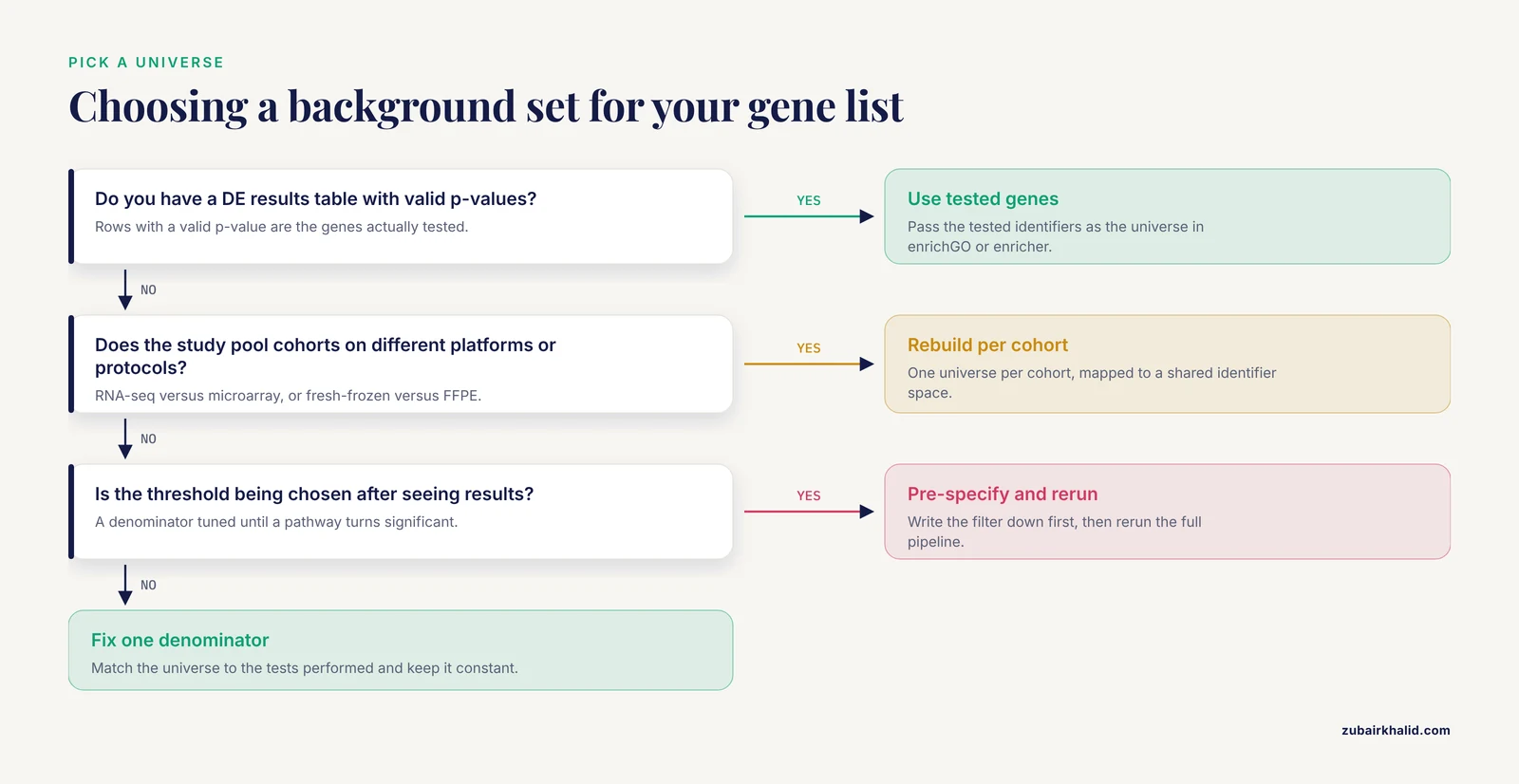
- Match the universe to the tests performed. If a gene had no chance to appear in your list, it does not belong in the denominator. The results table from your DE step is the cleanest definition.
- One universe per comparison. Upregulated and downregulated lists, and all contrasts in a study, should share a single universe. Different denominators make results incomparable.
- Pre-specify the filter. Choose the expression filter before running anything, write it down, and resist the urge to adjust it when a favorite pathway lands at q equal to 0.06.
- Keep set sizes sane and remember effective size. Sets below about 10 genes are unstable and sets above about 500 are nonspecific. Correlated members reduce the independent information in a set, so a 200-gene set with strong internal correlation behaves like a much smaller one.
- Handle direction explicitly. Run up and down lists separately against the same universe, or use ranked methods that take direction from the statistic. Combining directions in one list lets opposing genes cancel inside a set.
- Think about what the contrast means. A dual-comparison design in severe acute pancreatitis used SAP versus healthy controls to capture broad disease-associated changes and SAP versus mild disease to isolate organ-failure-associated features [6]. The list definition changes with the contrast, and the universe should stay constant so the lists remain comparable.
- Report the universe. The filter rule, the universe size, the identifier space, the gene set database with version and download date, and the set size limits. A reviewer should be able to reproduce your denominator from your methods section alone.
- When in doubt, rerun with the second most defensible universe. If conclusions survive both the tested-genes universe and a filtered expressed-genes universe, they are robust. If they flip, you have learned something about your result.
Worked Scenarios from RNA-seq Studies
Scenario 1: Bulk RNA-seq DEGs with Over-Representation Analysis
A gastric RNA-seq study of loperamide-induced dysmotility defined its DEG list as genes with fold change of at least 1.5 and false discovery rate (FDR), the adjusted p-value controlling the expected proportion of false positives, below 0.01. That produced 1,356 DEGs, 553 upregulated and 803 downregulated, followed by GSEA to characterize the involved pathways [7]. To reproduce the ORA half of such an analysis with a correct background:
- Start from raw counts, not normalized values.
- Filter low-count genes, for example keep genes with CPM above 1 in at least two samples.
- Run DESeq2.
- Define tested genes as rows with a valid p-value.
- Define the DEG lists with the pre-specified thresholds.
- Run ORA once per direction, passing the same tested set as the universe both times.
library(DESeq2)
library(clusterProfiler)
library(org.Hs.eg.db)

# after building the dds object from raw counts
dds <- DESeq(dds)
res <- results(dds, contrast = c("treatment", "loperamide", "vehicle"))

tested <- rownames(res)[!is.na(res$pvalue)]
deg_up <- rownames(res)[!is.na(res$padj) & res$padj < 0.01 &
                        res$log2FoldChange > log2(1.5)]
deg_down <- rownames(res)[!is.na(res$padj) & res$padj < 0.01 &
                          res$log2FoldChange < -log2(1.5)]

ego_up <- enrichGO(gene = deg_up, universe = tested,
                   OrgDb = org.Hs.eg.db, keyType = "ENSEMBL",
                   ont = "BP", pAdjustMethod = "BH",
                   minGSSize = 10, maxGSSize = 500)
If you skip step 4 and let the tool default to the full annotation, the 1,356-gene list is compared against a genome that includes transcripts your poly(A) library never quantified and genes your filter discarded. The p-values change, and nothing in the output warns you.
Scenario 2: GSEA on a Full Ranked List
A selenium nutrition study in rat liver illustrates why ranked methods exist and where their background decision actually lives. In earlier work, no single liver transcript was consistently and significantly altered by high selenium at q below 0.05, yet GSEA over the ranked transcript list found that deficiency downregulated the selenoprotein gene set and that the 5 µg Se/g diet upregulated 27 gene sets relative to the adequate diet [8]. The ranked list contained everything the platform measured, so the practical background decision was made upstream, at quantification and at any pre-ranking filter. This is also the case that justifies the ranked-list family, because coordinated shifts of modest size across many genes can carry a clear set-level signal even when no individual gene passes a per-gene threshold.
Scenario 3: Cross-Platform and FFPE Validation
When discovery and validation happen on different platforms, each cohort needs its own detectable gene space. A neuroblastoma study used RNA-seq from the TARGET cohort (n = 153) as its discovery set and two microarray cohorts (n = 498 and n = 223) for validation, applying GSEA within that design [9]. An aging-related lung adenocarcinoma study derived DEGs from The Cancer Genome Atlas (TCGA) and intersected them with two Gene Expression Omnibus (GEO) cohorts, GSE37745 and GSE50081, before building its signature [10]. In both designs, carrying one cohort's universe into the other would have been wrong, because the platforms measure different transcript spaces.
Fixation adds the same logic within a single platform. Poly(A) protocols are incompatible with FFPE RNA while ribosomal RNA depletion handles degraded material [1], and yet matched fresh-frozen and FFPE RNA-seq preserved molecular subtype calls in 91% of evaluable triple-negative breast cancer samples [11]. Robust downstream calls and a shifting detectable gene space can coexist, which is exactly why the universe should be rebuilt per protocol and reported per result.
Scenario 4: Single-Cell and Score-Based Analyses
In single-cell RNA-seq, quality control removes cells and genes, so the detectable gene space is matrix-specific and often much smaller than in bulk. Two lessons follow. First, fix the gene space after QC and use the same space for every scoring method you apply. A single-cell study of atopic dermatitis skin found that differences in disease-associated gene set scores between patient and healthy endothelial cells were small and inconsistent between scoring approaches [12], and that the endothelial module overlapping the disease gene set did so through only 10 genes at roughly 30-fold enrichment [12], a reminder that set definitions themselves shape what the background means. Second, treat score-based results as hypothesis-generating. An integrative study of diabetic retinopathy and Parkinson's disease ran both GSEA and gene set variation analysis (GSVA), which scores sets per sample, to triangulate shared pathways [13]. In both cases, the universe question became a preprocessing question, decided when the expression matrix was built.
Common Mistakes and Limitations
Most bioinformatics troubleshooting for enrichment results ends in the same place, a universe that does not match the list. The mistakes below account for the majority of reruns and reviewer objections.
Mistakes That Distort Enrichment Results
- Using the DEG list as its own background. Every set gene in the list is also in the universe by construction, the test degenerates, and the output is meaningless.
- Trusting the tool default. Many tools fall back to all genes in the annotation database or the GMT file when you omit the universe. After heavy filtering, that default is wrong.
- Mapping the list but not the universe. The tool then compares a mapped list against an unmapped denominator, and the arithmetic fails silently.
- Different universes for up and down lists, or across cohorts. The two directions stop being comparable, and cross-cohort contrasts become uninterpretable.
- Tuning the filter after seeing results. A denominator adjusted until the favorite pathway turns significant is not an analysis, it is a decision dressed as one.
- Carrying a universe across platforms or sample types. An RNA-seq universe does not transfer to a microarray validation cohort, and a fresh-frozen universe does not transfer to FFPE.
- Not reporting the universe. Without the filter rule and universe size, no one, including you six months later, can reproduce the result.
- Merging public datasets without a sample audit. In a pulmonary arterial hypertension study, a sample-title audit identified 68 shared sample identifiers between two GEO datasets, so the merged data represented 257 expression profiles from 189 unique subjects [14]. Duplicates distort group sizes, and group sizes feed every downstream test, including enrichment.
- Overreading borderline calls. In a three-cohort reanalysis of adhesive capsulitis, extracellular matrix remodeling was the clear signal, with a normalized enrichment score (NES) of 2.299 and q of 0.001, while necroptosis was lower at q of 0.035 and ferroptosis was borderline at q of 0.056 [15]. Report the statistics, label the borderline calls as borderline, and let readers see the difference between a clean hit and a maybe.
A Troubleshooting Checklist
- Every set comes back significant. The universe is too small, often the list itself, or identifier mapping collapsed it.
- Nothing comes back significant. The universe is too large, the sets shrank below the minimum size after mapping, or the list itself is too small.
- A set shows zero expected genes yet a p-value appears. The list and the universe live in different identifier spaces.
- Up and down results are not comparable. They were run with different universes, rerun both with one shared universe.
- Conclusions flip when the threshold moves. The filter was chosen post hoc, pre-specify it and rerun the full pipeline.
Limitations
Enrichment analysis inherits the biases of its annotations, which overrepresent well-studied genes and lag new biology. Sets overlap, so significant terms are not independent pieces of evidence. Competitive tests answer a narrow question, whether a set is overrepresented relative to the measured background, not whether the set matters biologically. No background choice rescues a weak list, a small sample size, or a contrast that fails to isolate the effect you care about. Treat the output as hypotheses and test them, as in a colorectal cancer study where GSEA implicated MYC target enrichment in lncRNA-driven malignancy and western blotting confirmed the mechanism [16]. Individual results also need domain judgment about which pathways are plausible for the tissue and treatment studied.
Frequently Asked Questions
What is the best background set for enrichment analysis in RNA-seq?
The best background set is the group of genes your differential expression step actually tested, meaning the rows of the results table with a valid p-value. If that table is unavailable, a pre-specified expressed-gene filter such as counts per million above 1 in at least two samples is the standard fallback. Avoid the whole-genome default and never use the DEG list itself.
Can I use the whole genome as the background for RNA-seq enrichment analysis?
Only as a rough exploratory default. A whole-genome background counts genes that poly(A) selection cannot capture and genes your expression filter removed, so the denominator describes an experiment you did not run. Reserve it for microarray-style data where the platform interrogates most genes, or for a first look you plan to rerun properly.
Do GSEA and ssGSEA need a background set?
They take no universe argument because the ranked list or expression matrix is the background. Your job is to control what enters it, which means deciding quantification scope, pre-ranking filters, and annotation mapping before you look at results, then keeping those choices fixed across all comparisons.
Should upregulated and downregulated gene lists share the same background?
Yes. Both lists come from the same tested gene space, so both should be tested against the same universe. Different universes make the two directions incomparable and are a common source of reviewer objections.
How does library preparation change the background?
Poly(A) capture misses non-polyadenylated transcripts and degraded material and is incompatible with FFPE RNA, while ribosomal RNA depletion retains a broader transcript space. Two libraries from the same tissue can therefore have different detectable gene spaces, so define the universe from your own quantified genes rather than from a generic annotation.
How should I report the background set in a paper?
Report the filter rule, the resulting universe size, the identifier space, the gene set database with version and download date, and the set size limits. A reviewer should be able to reproduce your denominator from that single sentence in the methods section.
Sources
- Comparison of RNA-Seq by poly (A) capture, ribosomal RNA depletion, and DNA microarray for expression profiling.
- Roastgsa: a comparison of rotation-based scores for gene set enrichment analysis.
- Identification and validation of circadian rhythm-related diagnostic biomarkers for endometriosis through integrating machine learning and single-cell analysis.
- Single-Cell RNA Sequencing-Integrated Fibroblast Markers and Candidate Drug-Target Associations in Pancreatic Ductal Adenocarcinoma.
- Transcriptome analysis of sevoflurane exposure effects at the different brain regions.
- Integrative transcriptomic analysis of peripheral blood identifies NETosis-associated programs and a stratified adaptive immune suppression pattern in severe acute pancreatitis.
- Transcriptomic insights into loperamide-induced gastric dysmotility: RNA-seq analysis of a mouse model.
- Gene Set Enrichment Analysis of Selenium-Deficient and High-Selenium Rat Liver Transcript Expression and Comparison With Turkey Liver Expression.
- Comparison of Stage 4 and Stage 4s Neuroblastoma Identifies Autophagy-Related Gene and LncRNA Signatures Associated With Prognosis.
- Integrated analysis identifies an aging-related prognostic signature for lung adenocarcinoma.
- Comparison of triple-negative breast cancer molecular subtyping using RNA from matched fresh-frozen versus formalin-fixed paraffin-embedded tissue.
- Integrative Single-Cell Transcriptomic Analysis Identifies Candidate Endothelial Activation Signatures in Atopic Dermatitis.
- An Exploratory Single-Cell Analysis Identifies Candidate Shared Molecular Features in Proliferative Diabetic Retinopathy and Parkinson's Disease.
- Integrative single-cell and bulk transcriptomic analysis identifies monocyte/macrophage senescence-associated candidate genes in pulmonary arterial hypertension.
- Extracellular matrix remodeling and regulated cell-death-immune associations in adhesive capsulitis: a three-cohort transcriptomic analysis.
- Long non-coding RNA RP3-380B8.4 facilitates tumor malignancy, liver metastasis and shapes an immunosuppressive tumor microenvironment in colorectal cancer.