Cost-Effective Autoscaling for Bioinformatics Pipelines
By Dr. Zubair Khalid, DVM, MS, PhD ·

By the end of this guide you will be able to configure a Nextflow pipeline that runs on AWS Batch, scales automatically from zero vCPUs up to hundreds during a run and back down to zero when it finishes, uses Spot instances safely, and can be priced with a simple formula before you launch it. You will also be able to apply the same reasoning on Google Cloud Platform, on a managed Kubernetes service, and in a hybrid HPC plus cloud setup.
What you need on hand before starting:
- An AWS account with permissions for EC2, Batch, S3, and IAM, plus the AWS CLI version 2 installed and configured with
aws configure - A working pipeline in Nextflow, Snakemake, or WDL/Cromwell, packaged tasks as Docker or Singularity images
- An S3 bucket for inputs, intermediates, and outputs
- Rough per-task resource numbers for your workload, meaning vCPUs, memory, and wall-clock time per sample
The core idea behind autoscaling bioinformatics cost control is simple. Sequencing workloads are bursty. A pipeline that processes 300 samples spends most of its life in embarrassingly parallel per-sample steps, then drops back to near-idle between batches. A cluster that sits idle between runs burns money for nothing, while a fixed-size cluster that is too small stretches your turnaround for no reason. Autoscaling, which means automatically growing and shrinking the compute fleet to match the number of queued tasks, lets you pay for compute only in the minutes it is actually working. Published benchmarks put real numbers on this: a cloud curation of more than 126,000 CT volumes used more than 21,000 virtual machines, finished in under 9 hours instead of an estimated 522 days on one workstation, and cost $1,011.05 in total [1]. Another team quantified transcript expression for 12,307 RNA-seq samples using preemptible virtual machines for as little as $0.09 per sample [2]. That is the ceiling of what disciplined autoscaling buys you.
Why Cloud Bioinformatics Workloads Are Ideal for Autoscaling
Most sequencing pipelines are what workflow engines call scatter and gather. The scatter phase runs the same CPU-bound task independently across every sample in the cohort, for example BWA-MEM alignment or FastQC. The gather phase reduces those outputs, often with a small number of larger, memory-hungry jobs such as joint genotyping. Between runs, the cluster does nothing.
Three properties make this pattern cheap in the cloud if you scale correctly:
- Parallelism is per sample. Two hundred samples means two hundred independent tasks, which maps cleanly onto an autoscaling fleet.
- Tasks are short and stateless. Most per-sample steps run for minutes to hours and read and write to object storage, so any instance can pick up any task.
- The data already lives in the cloud. Public compendia are measured in petabytes, which makes transferring data to a local computer infeasible and favors bringing tools to the data [2]. The UK Biobank Research Analysis Platform follows the same compute-to-data model for whole-genome sequencing analysis [3].
The alternative, a fixed on-premise cluster sized for your largest project, sits underutilized most of the year. The alternative in the cloud, a fixed-size cluster you forgot to scale down, is worse because you pay for idle vCPUs at retail. Autoscaling from zero is the setting that fixes both problems.
The Cost Model to Build Before You Scale Anything
Before touching a compute environment, write down where your money actually goes. A detailed cost breakdown for a cloud personal-genome pipeline separated spending into storage, compute, and I/O, and projected those three categories for large datasets [4]. That three-way split is the right mental model for any cloud bioinformatics project.
Compute cost follows a simple formula:
compute_cost = Σ over tasks ( vCPUs_per_task × hours × vCPU_hour_price )For a homogeneous fleet this collapses to:
compute_cost = instance_hours × price_per_instance_hourStorage cost accrues every hour that data sits in S3, EBS snapshots, or Glacier, including intermediates you forgot to clean up. I/O cost includes data transfer between availability zones, egress out of the cloud, and repeated reads of large reference files if you do not cache them.
Worked example. Suppose a per-sample variant calling step needs 4 vCPUs and 6 hours, and you have 200 samples:
total vCPU-hours  = 200 × 4 × 6      = 4,800 vCPU-hours
on a 4-vCPU instance type:
instance-hours    = 4,800 / 4        = 1,200 instance-hours
cost              = 1,200 × P        (P = your region's hourly price for that instance)
Now compare the two failure modes. If you run a fixed 50-instance cluster for a month so the project can start instantly at any time:
idle_cluster_cost = 50 × 730 × P = 36,500 × PAutoscaling from zero costs 1,200 × P for the same work. Even at a very cheap hourly rate, the difference between 1,200 instance-hours and 36,500 instance-hours is the entire economic argument for autoscaling in cloud bioinformatics. The formula also shows why benchmarking matters, because P is fixed but the instance-hours term is entirely under your control through batching, instance sizing, and algorithm choice [5].
Step-by-Step: Autoscaling a Nextflow Pipeline on AWS Batch
This walkthrough uses Nextflow with the awsbatch executor, which is the standard setup for AWS genomics workloads. The same parameter logic applies to Cromwell on Batch and to Snakemake running inside a container on Batch or Kubernetes.
Step 1. Stage data and tag resources
Put inputs in S3 and apply a cost-allocation tag so Cost Explorer can attribute your spending:
aws s3 sync ./cohort/ s3://mylab-wgs-2026/fastq/ \
  --storage-class STANDARD

aws s3api put-object-tagging \
  --bucket mylab-wgs-2026 \
  --key fastq/sample001_R1.fastq.gz \
  --tagging 'TagSet=[{Key=Project,Value=wgs-cohort-2026}]'
Step 2. Create a Spot-backed compute environment that scales to zero
Save this as spot-ce.json. The three values that control autoscaling bioinformatics cost are minvCpus, desiredvCpus, and maxvCpus:
{
  "computeEnvironmentName": "nf-spot-ce",
  "type": "MANAGED",
  "state": "ENABLED",
  "computeResources": {
    "type": "SPOT",
    "allocationStrategy": "SPOT_CAPACITY_OPTIMIZED",
    "instanceTypes": ["m5.xlarge", "m5.2xlarge", "m5a.2xlarge", "m5ad.2xlarge"],
    "minvCpus": 0,
    "desiredvCpus": 0,
    "maxvCpus": 512,
    "instanceRole": "arn:aws:iam::123456789012:instance-profile/ecsInstanceRole",
    "spotIamFleetRole": "arn:aws:iam::123456789012:role/spot-fleet-role",
    "bidPercentage": 90
  },
  "serviceRole": "arn:aws:iam::123456789012:role/batch-service-role"
}
Create it and attach a job queue:
aws batch create-compute-environment \
  --cli-input-json file://spot-ce.json

aws batch create-job-queue \
  --job-queue-name nf-spot-queue \
  --state ENABLED \
  --priority 1 \
  --compute-environment-order order=nf-spot-ce,position=1
Expected output for the first command is a JSON document with "computeEnvironmentName": "nf-spot-ce" and "status": "VALID". If you see "status": "CREATING", wait a minute and run aws batch describe-compute-environments, compute-environments nf-spot-ce until it reports VALID.
Parameter meanings:
minvCpus: 0lets the fleet shrink to nothing when the queue is empty. This is the single most cost-relevant setting. A nonzero minimum means you pay 24 hours a day whether or not you are analyzing anything.desiredvCpus: 0starts with no running instances. Batch raises this automatically as jobs are submitted.maxvCpus: 512caps the blast radius. With 16-vCPU instances, this is up to 32 concurrent instances. Set it to a number you would be comfortable seeing on a bill for one long day.allocationStrategy: SPOT_CAPACITY_OPTIMIZEDasks EC2 to draw from Spot pools with the lowest chance of interruption, which reduces the retry churn that wastes partial compute.bidPercentage: 90refuses to launch instances priced above 90 percent of on-demand, protecting you from the rare high Spot prices.
Step 3. Configure the pipeline for retry-safe Spot execution
Spot instances are reclaimed with about two minutes of notice, which kills any running task. Your workflow engine must treat that as a retryable event. In nextflow.config:
process {
  executor      = 'awsbatch'
  queue         = 'nf-spot-queue'
  errorStrategy = 'retry'
  maxRetries    = 4

  withLabel:process_medium {
    cpus   = 4
    memory = 16.GB
  }
  withLabel:process_high {
    cpus   = 16
    memory = 64.GB
  }
}

aws {
  region = 'us-east-1'
  batch {
    maxParallelTransfers = 16
  }
}
errorStrategy = 'retry' combined with maxRetries is what makes Spot viable. When AWS Batch marks an interrupted job as failed, Nextflow resubmits it and any available instance picks it up. Each retry re-downloads the input from S3 and re-runs the task from scratch, which is cheap for per-sample steps but is a reason to keep long gather steps on larger, more stable instances where possible.
Step 4. Launch and watch the fleet scale
nextflow run nf-core/sarek \
  -profile test \
  -w s3://mylab-wgs-2026/work \
  -resume
In a second terminal, watch the autoscaler work:
watch -n 30 'aws batch describe-compute-environments \
  --compute-environments nf-spot-ce \
  --query "computeEnvironments.computeResources.[minvCpus,desiredvCpus,maxvCpus]" \
  --output text'
Expected output during the scatter phase looks like:
0 176 512and after the pipeline drains, back to:
0 0 512If the middle number never rises, the queue name in nextflow.config does not match the queue you created. If it rises but jobs stay in RUNNABLE, your instanceRole or spotIamFleetRole is wrong, or no Spot capacity of the requested types exists in that region, which you fix by broadening the instanceTypes list.
Step 5. Verify what you actually spent
Tag-based cost attribution in Cost Explorer, or the CLI equivalent:
aws ce get-cost-and-usage \
  --time-period Start=2026-10-01,End=2026-11-01 \
  --granularity DAILY \
  --metrics UnblendedCost \
  --group-by Type=TAG,Key=Project \
  --query "ResultsByTime[].{Day:TimePeriod.Start, Cost:Total.UnblendedCost.Amount}"
Expected output is one line per day, for example:
[
  { "Day": "2026-10-14", "Cost": "38.42" },
  { "Day": "2026-10-15", "Cost": "51.09" },
  { "Day": "2026-10-16", "Cost": "0.00" }
]
A flat near-zero tail after the run ends is your confirmation that the fleet scaled back to zero. A persistent daily charge after jobs finish almost always means an unattached EBS volume, an idle NAT gateway, or a leftover EC2 instance outside Batch.
Step 6. Clean up intermediates
aws s3 rm s3://mylab-wgs-2026/work/ --recursive \
  --exclude "*.bam" --exclude "*.vcf.gz"
Deleting the work directory of per-sample intermediates is the cheapest bill reduction available, because it stops hourly storage accrual on objects you will never read again.
Tuning the Parameters That Move the Bill
Once the walkthrough works, four levers dominate autoscaling bioinformatics cost in practice.
Strategic batching. Benchmarking of the GenomeKey whole-genome workflow on AWS identified strategic batching of individual genomes and efficient cluster resource configuration as key levers for fast, scalable, low-cost clinical-grade analysis [5]. In Nextflow terms, this means deciding how many samples each job processes. A job per sample maximizes parallelism but pays instance-start overhead 200 times. Batching 8 to 16 samples per job amortizes startup and reference loading, at the cost of longer task runtime and coarser retries. Benchmark both on your cohort before choosing.
Right-sizing resource hints. Every task that requests 16 vCPUs but uses 4 wastes 75 percent of an instance-hour. Collect actual peak memory and CPU from completed runs (Nextflow reports them in the trace file) and set process labels from measured values, not from what the tool documentation suggests.
Algorithm and architecture choices. A UK Biobank fine-mapping study on whole-genome sequencing data reported a 44 percent cost reduction and a 94 percent speedup through compute architecture optimization alone, with no change in scientific output [3]. Distributed reimplementations of core steps can shift the curve further. A cloud-native distributed pileup implementation was up to 6.5 times faster and used up to 2 times less memory than other distributed tools, which the authors attribute directly to substantial cloud cost reduction [6]. Before buying more vCPUs, check whether a better partitioned version of your bottleneck step exists.
Instance family breadth. Listing three to five instance families across generations in instanceTypes increases Spot availability and lowers interruption frequency. Mixing m5, m5a, and m5ad classes is more resilient than pinning one type.
Spot, On-Demand, and Managed Autoscaling Compared
The table below summarizes the options that matter for cost-effective autoscaling of bioinformatics pipelines, including the formulas from the cost model above.
| Option or parameter | What it does | Cost behavior | When to use |
|---|---|---|---|
| On-demand instances | Fixed hourly rate, no interruption risk | Highest hourly price, full predictability | Short gather steps, deadlines, small pilot runs |
| Spot instances | Spare capacity at a large discount, reclaimable with short notice | Typically the lowest hourly cost, plus retry overhead | Scatter-phase per-sample tasks with errorStrategy = retry |
| Autoscaling managed fleet (min 0) | Grows with queue depth, shrinks to zero when idle | Pay only for active task time plus brief launch lag | Default for all cloud bioinformatics batch work |
| Reserved capacity or savings commitments | Commitment in exchange for a lower rate | Lower hourly price, obligation regardless of use | Steady baseline load such as always-on databases, not burst pipelines |
| Cost formula | compute_cost = task_vCPUs × hours × vCPU_price, summed over tasks | Linear in total vCPU-hours | Pre-launch budgeting and comparing batch sizes |
A useful pre-launch habit is to compute both instance_hours × price for the autoscaled plan and peak_instances × 730 × price for the fixed-cluster alternative. The gap is your documented savings, which helps when justifying cloud spend to a grant administrator.
What Published Benchmarks Say About Cluster Size and Speed-Cost Tradeoffs
Configuring cluster size by intuition is a common failure. Several peer-reviewed benchmarking studies give you empirical anchors.
For population-scale genomics, researchers ran GWAS on Spark clusters with the Hail framework on both Google Cloud Platform and Amazon Web Services, across four whole-genome sequencing datasets. Comparing many cluster configurations produced a clear compromise between speed and cost, and the results were consistent across both providers [7]. Two lessons carry over directly. First, the fastest configuration is almost never the cheapest, so benchmark several node counts and record dollars per completed analysis. Second, because the ranking of configurations held across two providers, you can benchmark on one cloud and trust the shape of the curve elsewhere.
For whole-genome clinical pipelines, the GenomeKey study on AWS used systematic benchmarking of the COSMOS workflow manager to reach turnaround in hours at economies in the tens of dollars per genome, with batching and cluster configuration as the decisive variables [5]. Their methodology, sweeping task size and cluster shape and plotting cost per genome, is reproducible with any modern workflow engine.
For assemblers and other locality-heavy workloads, a Hadoop and Giraph based assembler achieved high scalability over hundreds of compute nodes by collocating computation with data, and performed better on SSD-based cloud infrastructure than on a traditional cluster, with strong results at 256 cores [8]. The general principle is that I/O character determines the optimal fleet shape. Alignment and pileup workloads that read large BAM partitions need fast local or network storage, while per-sample QC tasks do not.
For GPU-accelerated callers, DeepVariant-on-Spark added Spark-based resource allocation and multi-GPU support to DeepVariant, deployed on Google Cloud Platform, where the authors state a user can go from nothing to analyzing at least ten whole-genome datasets within 20 minutes of setup using free credits [9]. This is a reminder that the right unit of autoscaling is not always a vCPU. For deep-learning variant calling, the fleet scales in GPUs and the cost formula gains a GPU-hour term.
Scheduling and Bidding Strategies That Go Beyond Manual Tuning
Once manual tuning plateaus, there is a published literature on automated allocation.
Linear programming over Spot markets. Aether used linear programming to optimally bid on and deploy combinations of underutilized cloud resources, simultaneously minimizing analysis cost while easing the transition from existing HPC pipelines [10]. The practical takeaway for teams not ready to adopt an LP solver is directional. Rather than bidding on one instance type, spread demand across many instance families and sizes, and let a scheduler pick the cheapest feasible combination for each task.
Metaheuristic task placement. A study of epigenomics scientific workflows on cloud platforms applied an improved particle swarm optimization algorithm to map tasks to resources, reducing total workflow cost by 6.83 percent compared with the traditional algorithm [11]. A 6.83 percent saving from scheduling alone, on top of instance selection, illustrates how much headroom exists between naive round-robin placement and cost-aware placement.
Load balancing across HPC and cloud. clubber automated the balancing of parallel submissions across available HPC resources, which can be extended on demand with cloud nodes in heterogeneous environments, and processed 21 metagenomes in 172 minutes in their demonstration [12]. This matters if your lab already owns an HPC queue. The cost-effective pattern is to keep the HPC busy first and let the autoscaled cloud fleet absorb only the overflow, because the marginal cost of owned, depreciated hardware is near zero while every cloud vCPU-hour bills.
Platform-level optimization. The RAPpoet approach on the UK Biobank Research Analysis Platform, mentioned above, is an example of optimizing compute architecture inside a managed platform rather than rebuilding the stack [3]. If your data is already hosted on a managed genomics platform, optimizing job shape and instance selection inside that platform is usually cheaper than migrating.
Hybrid and Multi-Cloud Patterns
Autoscaling does not require everything to live in one public cloud.
Hybrid cloud microservices. The SenNet Data Portal, which hosts over 1,700 public human and mouse datasets across 15 organs, runs on a scalable hybrid cloud microservices architecture serving 13 tissue mapping centers and 12 technology development components [13]. For portal-style services with steady baseline traffic plus bursty analysis demand, the hybrid pattern is to run the always-on components on reserved capacity or on-premise hardware and autoscale the bursty analysis components into Spot capacity.
Hybrid execution models inside one pipeline. Closha combines traditional workflow tools and MapReduce-based big data programs in a single pipeline, letting analytical algorithms be parallelized where appropriate, and adds a dedicated high-speed transfer solution [14]. The design point is worth copying: not every step in a genomics pipeline benefits from the same execution engine, and letting per-step engines differ often beats forcing one paradigm.
Community clouds and SaaS. The Atlas2 pipeline was deployed both on a community cloud through the Genboree Workbench and commercially on AWS as software-as-a-service, with a published cost structure covering storage, compute, and I/O [4]. For small labs, a community cloud or hosted SaaS can deliver autoscaling without requiring anyone on staff to maintain IAM roles and Batch queues.
Common Mistakes and Limitations
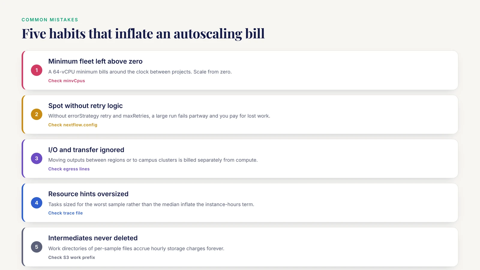
These are the errors that most often turn a well-designed autoscaling setup into an expensive one.
- Leaving
minvCpusabove zero. A minimum fleet of 64 vCPUs bills around the clock, every day, between projects. Scale from zero unless something in your architecture genuinely requires a warm fleet. - Running Spot without retries. Spot instances are reclaimed with short notice. Without
errorStrategy = 'retry'and a healthymaxRetries, a large scatter-gather run fails partway and you pay for the lost partial work. The retry strategy is what converts Spot's discount into a real saving. - Ignoring I/O and transfer costs. The Atlas2 cost analysis treated storage and I/O as first-class budget lines alongside compute [4]. Copying the same reference files into 200 instance-local disks is usually fine, but moving outputs between regions or out to campus clusters is billed separately and can quietly rival compute cost on small projects.
- Oversizing memory and CPU hints. Tasks sized for the worst sample rather than the median sample inflate the instance-hours term of the cost formula. Measure per-task peaks and set labels from the distribution.
- Forgetting to delete intermediates. Work directories full of per-sample intermediates accrue hourly storage charges forever. Schedule deletion as part of the pipeline's final step, as in the walkthrough above.
- Assuming published configurations transfer directly. The GWAS benchmarking study found a clear speed-cost compromise, but one derived from their specific datasets and cluster configurations [7]. Treat published numbers as hypotheses and rerun a small benchmark sweep on your own cohort before committing.
- Chasing parallelism when the algorithm is the problem. The UK Biobank work showed 44 percent cost savings from architecture optimization rather than from adding instances [3], and the distributed pileup work showed the same effect at the single-step level [6]. If one step dominates the bill, optimize that step before scaling the fleet larger.
- Treating autoscaling as free fault tolerance. Retries re-run work from scratch, so each Spot interruption costs the partial runtime of the killed task. On very long single tasks, batching more samples per job or placing the step on stable capacity can cost less overall.
- No cost attribution. Without tags and periodic Cost Explorer review, the first sign of a misconfigured compute environment is a monthly invoice. The daily cost query in the walkthrough takes a minute to run and catches idle fleets, orphaned volumes, and runaway maxima.
An honest limitation: every precise number in this article comes from specific studies on specific datasets and pricing eras. Cloud list prices change, Spot markets fluctuate hourly, and your pipeline's cost profile is yours alone. The formulas and the benchmarking procedure transfer, the absolute dollars do not.
Frequently Asked Questions
What is autoscaling in a bioinformatics pipeline?
Autoscaling means the compute fleet automatically grows when your workflow engine submits tasks and shrinks toward zero when the queue empties, so you pay for capacity only while it is running work. In cloud bioinformatics this is implemented with managed fleets such as AWS Batch compute environments or Kubernetes node pools.
How much money can cost-effective autoscaling actually save?
It eliminates idle-cluster spend, which in the worked example above is the difference between 1,200 billed instance-hours for the actual work and 36,500 billed instance-hours for a fixed fleet kept warm for a month. Published projects also report large savings from combining autoscaling with Spot pricing and architecture optimization, so the total effect is often a large multiple of the naive fixed-cluster cost.
Should I use Spot or on-demand instances for genomics pipelines?
Use Spot for the embarrassingly parallel per-sample steps, with automatic retries configured, and on-demand for short, deadline-critical, or hard-to-retry gather steps. That split captures most of the discount while limiting the cost of any single interruption.
What should minvCpus, desiredvCpus, and maxvCpus be set to?
Set minvCpus to 0 and desiredvCpus to 0 so the fleet scales to zero between runs, and set maxvCpus to the largest number you would be comfortable paying for in a single day. Then verify with a Cost Explorer query that costs return to zero after each run.
Do these methods work with Nextflow, Cromwell, and Snakemake?
Yes. Nextflow with the awsbatch executor, Cromwell on AWS Batch, and Snakemake on Batch or Kubernetes all rely on the same underlying autoscaling fleet, so the compute environment settings, retry strategy, and cost formulas in this guide apply to all three.
What are the most common mistakes that inflate autoscaling bills?
The leading causes are a nonzero minimum fleet size, Spot execution without retry logic, untracked storage and transfer charges, resource hints far above measured task needs, and never deleting intermediate files. All five are checkable in under an hour on an existing project.
Which cloud providers are best for AWS genomics and related work?
AWS and Google Cloud Platform are both well established for genomics workloads, and a comparative GWAS benchmarking study found that the ranking of speed-versus-cost configurations was consistent across the two providers [7]. Choose based on where your data already lives, because bringing compute to the data avoids large transfer costs [2].
Can autoscaling work with an on-premise HPC cluster?
Yes. The cost-effective pattern is load balancing across the HPC queue first and bursting overflow into an autoscaled cloud fleet, which is the model demonstrated by cluster-load-balancing systems for big data bioinformatics [12]. Reserved or owned hardware handles the baseline, and Spot-backed cloud capacity absorbs the peaks.
Sources
- Cloud-based large-scale curation of medical imaging data using AI segmentation.
- A cloud-based workflow to quantify transcript-expression levels in public cancer compendia.
- Optimizing UK biobank cloud-based research analysis platform to fine-map coronary artery disease loci in whole genome sequencing data.
- Atlas2 Cloud: a framework for personal genome analysis in the cloud.
- Scalable and cost-effective NGS genotyping in the cloud.
- Cloud-native distributed genomic pileup operations.
- Scalability and cost-effectiveness analysis of whole genome-wide association studies on Google Cloud Platform and Amazon Web Services.
- Large-scale parallel genome assembler over cloud computing environment.
- DeepVariant-on-Spark: Small-Scale Genome Analysis Using a Cloud-Based Computing Framework.
- Aether: leveraging linear programming for optimal cloud computing in genomics.
- Cancer Diagnosis Epigenomics Scientific Workflow Scheduling in the Cloud Computing Environment Using an Improved PSO Algorithm.
- clubber: removing the bioinformatics bottleneck in big data analyses.
- SenNet Portal: Build, Optimization and Usage.
- Closha: bioinformatics workflow system for the analysis of massive sequencing data.