How to Automate a Simple RNA-Seq Analysis with a Bash Script

By Dr. Zubair Khalid, DVM, MS, PhD · 2026-11-11

By the end of this article you will have a working bash script that takes a folder of paired-end RNA-Seq FASTQ files and runs the entire analysis for you: quality control, adapter and quality trimming, splice-aware alignment to a reference genome, sorting and indexing of alignments, and gene-level read counting. You will also have a companion R script that turns the count matrix into a differential expression table with DESeq2. Every command is real and runnable, every parameter is explained, and the failure modes you are most likely to hit are listed with their exact error messages and fixes.

This article assumes a Linux environment and uses the core Linux commands bioinformatics work depends on every day. Nothing here requires root access on a shared server. If you have a computer or cluster account with about 16 GB of RAM, 50 GB of free disk space, and the conda package manager installed, you have everything you need.

Why Automate an RNA-Seq Workflow in Bash

A bulk RNA-Seq experiment produces billions of reads that must pass through the same chain of steps every time: quality control, trimming, alignment, filtering, counting, and statistical testing. Doing this by hand for even six samples means retyping nearly identical commands dozens of times, and each retyped command is a chance to point at the wrong file or forget a parameter. The reproducibility problem is well recognized. Many laboratories rely on in-house scripts, which makes standardization and reproducibility difficult across projects and analysts, and one response has been to package the whole chain of steps, from quality control through counting to differential expression, into automated pipelines that can run from the command line [1].

Bash is the right starting point for three reasons. First, every bioinformatics command-line tool is invoked from the shell anyway, so a bash script simply records the exact invocations you would have typed. Second, bash requires no new language to learn before you see results. Third, the discipline of writing a script forces you to make every choice explicit, which is precisely what makes an analysis reproducible. The same principle shows up across computational biology. The admixr package was created because a traditional workflow required generating text configuration files for each analysis through a mix of shell scripting and manual text editing, then parsing non-tabular output by hand. Automating all low-level configuration and parsing steps made each analysis a single command and significantly improved reproducibility [2]. Your bash script does the same job for RNA-Seq. It wraps the low-level steps so that the whole analysis becomes one command that behaves identically every time it runs.

What the Pipeline Does, Step by Step

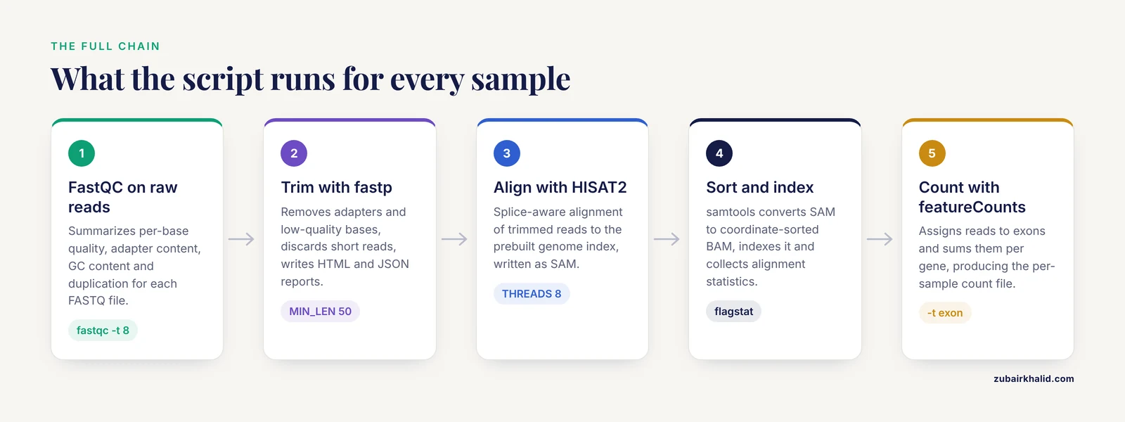
The workflow follows the standard bulk RNA-Seq structure described in standard textbooks and implemented by published pipelines [1]:

1. Quality control on raw reads. FastQC summarizes per-base quality, adapter content, GC content, and duplication for each FASTQ file.
2. Trimming and filtering. fastp removes adapters and low-quality bases, discards short reads, and writes its own HTML and JSON quality reports.
3. Splice-aware alignment. HISAT2 aligns trimmed reads to a reference genome, using a prebuilt genome index.
4. Sorting and indexing. samtools converts SAM output to coordinate-sorted BAM, indexes it, and collects alignment statistics.
5. Gene-level quantification. featureCounts from the Subread package assigns reads to exons and sums them per gene, producing the count matrix.
6. Quality aggregation. MultiQC scans the folder and combines all FastQC, fastp, and HISAT2 reports into one page.
7. Differential expression. A DESeq2 R script reads the count matrix, normalizes, models, and writes a table of results with adjusted p-values.

Each step is a small, independent program. The bash script is the glue that runs them in order, per sample, without manual intervention.

Step 1. Set Up Your Linux Environment for Bioinformatics

Linux for bioinformatics means two things in practice: a shell where commands run, and a package manager that installs tools without breaking each other. Conda solves the second problem through isolated environments.

Check what you have first:

which conda
conda --version
nproc
free -g
df -h .

nproc prints your CPU count, free -g shows RAM in gigabytes, and df -h . shows free disk space in the current directory. On a typical workstation you might see 8 CPUs, 32 GB of RAM, and several hundred gigabytes free. Write the CPU number down. You will feed it to the script as a variable.

Create a dedicated environment with every tool the pipeline needs:

conda create -n rnaseq -c conda-forge -c bioconda \
  fastqc=0.12.1 \
  fastp=0.24.0 \
  hisat2=2.2.1 \
  samtools=1.20 \
  subread=2.0.6 \
  multiqc=1.25 \
  wget

Activate it and verify each tool answers with a version banner:

conda activate rnaseq
fastqc --version
fastp --version
hisat2 --version | head -1
samtools --version | head -1
featureCounts -v
multiqc --version

Expected output looks like this (versions will match what you installed):

FastQC v0.12.1
fastp 0.24.0
hisat2 2.2.1
samtools 1.20
featureCounts v2.0.6
MultiQC v1.25

The -c bioconda channel is the standard source for bioinformatics software in conda. Pinning versions with = signs matters. A pipeline that runs against fastp 0.23 one month and fastp 0.25 the next is not reproducible, and the reproducibility argument for automation only holds if the software itself is fixed [2].

Step 2. Download a Reference Genome and Build an Index

HISAT2 needs two things: a genome FASTA file and a GTF annotation file that names exons and genes. For this walkthrough use the small, freely distributed Saccharomyces cerevisiae (baker's yeast) reference from the Saccharomyces Genome Database, or substitute any Ensembl genome you prefer. Yeast aligns and counts in minutes, which makes the pipeline fast to test. The same script works unchanged for human or mouse once you swap the files.

mkdir -p ~/rnaseq_tutorial
cd ~/rnaseq_tutorial
mkdir -p reference raw_data results logs scripts

cd reference
wget https://downloads.yeastgenome.org/sequence/S288C_reference/genome/S288C_reference_genome_R64-3-1_20230823/saccharomyces_cerevisiae_R64-3-1_20230823_genome.fsa
wget https://downloads.yeastgenome.org/sequence/S288C_reference/annotation/R64-3-1/saccharomyces_cerevisiae_R64-3-1_20230823.gff

mv saccharomyces_cerevisiae_R64-3-1_20230823_genome.fsa genome.fsa
mv saccharomyces_cerevisiae_R64-3-1_20230823.gff genes.gff

SAM and BAM coordinate systems and GFF/GTF gene annotation formats are standard textbook material, so a short orientation is enough. The FASTA file holds the chromosome sequences. The GFF file declares where each gene and exon sits on those chromosomes. featureCounts reads the GFF to decide which gene each aligned read belongs to.

Build the HISAT2 index and the samtools chromosome index:

hisat2-build -p 8 genome.fsa genome_index
samtools faidx genome.fsa

hisat2-build -p 8 uses 8 threads and writes several files all starting with genome_index. That prefix, not any single file, is what you pass to hisat2 later. samtools faidx creates genome.fsa.fai, a tiny index that tools use to fetch chromosome lengths. Building a yeast index takes under a minute. Building a human index takes roughly 30 to 60 minutes and about 8 GB of disk, which is why the index lives outside the per-sample loop and is built exactly once.

Verify the index was built:

ls -lh genome_index*

Expected output:

-rw-r--r-- 1 you you 3.3M Aug 23 2024 genome_index.1.ht2
-rw-r--r-- 1 you you 1.3M Aug 23 2024 genome_index.2.ht2
-rw-r--r-- 1 you you  77K Aug 23 2024 genome_index.3.ht2
-rw-r--r-- 1 you you  77K Aug 23 2024 genome_index.4.ht2
-rw-r--r-- 1 you you 3.3M Aug 23 2024 genome_index.5.ht2
-rw-r--r-- 1 you you 1.3M Aug 23 2024 genome_index.6.ht2
-rw-r--r-- 1 you you  12M Aug 23 2024 genome_index.7.ht2
-rw-r--r-- 1 you you  12M Aug 23 2024 genome_index.8.ht2

Eight .ht2 files means the index is complete. Fewer than eight means hisat2-build was interrupted and you must rebuild.

Step 3. Organize Raw Data and Write a Sample Sheet

Place paired-end FASTQ files in raw_data/ using a naming convention where the two mates of one sample share a prefix and differ by _1 and _2:

raw_data/
  WT_rep1_1.fastq.gz   WT_rep1_2.fastq.gz
  WT_rep2_1.fastq.gz   WT_rep2_2.fastq.gz
  WT_rep3_1.fastq.gz   WT_rep3_2.fastq.gz
  KO_rep1_1.fastq.gz   KO_rep1_2.fastq.gz
  KO_rep2_1.fastq.gz   KO_rep2_2.fastq.gz
  KO_rep3_1.fastq.gz   KO_rep3_2.fastq.gz

Then create a sample sheet. The sample sheet is the single source of truth for which samples exist, and the script reads it rather than guessing filenames. This avoids an entire class of bugs where a file is silently skipped.

cd ~/rnaseq_tutorial
cat > samples.csv << 'EOF'
sample_id
WT_rep1
WT_rep2
WT_rep3
KO_rep1
KO_rep2
KO_rep3
EOF

The script reconstructs both mate filenames from the sample ID, so the _1 and _2 naming convention is a requirement, not a suggestion. If your sequencing facility delivers names like sampleA_R1.fastq.gz, either rename the files or adjust the variable in the script.

Step 4. Write the Bash Script

This is the core of the article and the automate rna-seq bash script template you will reuse. Save it as scripts/run_rnaseq.sh inside the project folder.

#!/usr/bin/env bash
#
# run_rnaseq.sh
# Automate a simple bulk RNA-Seq analysis: QC, trimming, alignment,
# sorting, indexing, gene-level counting, and report aggregation.
#
# Usage:   bash scripts/run_rnaseq.sh
# Inputs:  samples.csv in the project root, raw_data/<sample>_1.fastq.gz
#          and raw_data/<sample>_2.fastq.gz for every sample ID listed.

set -euo pipefail

# ------------------------------------------------------------------
# Configuration. Edit these lines for your project.
# ------------------------------------------------------------------
PROJECT_DIR="$HOME/rnaseq_tutorial"
REF_DIR="$PROJECT_DIR/reference"
HISAT2_INDEX="$REF_DIR/genome_index"
ANNOTATION="$REF_DIR/genes.gff"
THREADS=8
MIN_LEN=50
MEAN_QUAL=20
STRANDEDNESS=0        # 0 = unstranded, 1 = stranded, 2 = reversely stranded

RAW_DIR="$PROJECT_DIR/raw_data"
TRIM_DIR="$PROJECT_DIR/results/trimmed"
ALIGN_DIR="$PROJECT_DIR/results/aligned"
COUNT_DIR="$PROJECT_DIR/results/counts"
LOG_DIR="$PROJECT_DIR/logs"
SAMPLE_SHEET="$PROJECT_DIR/samples.csv"

mkdir -p "$TRIM_DIR" "$ALIGN_DIR" "$COUNT_DIR" "$LOG_DIR"

log() {
    printf '[%s] %s\n' "$(date '+%Y-%m-%d %H:%M:%S')" "$*"
}

# ------------------------------------------------------------------
# Read the sample sheet, skipping the header line.
# ------------------------------------------------------------------
mapfile -t SAMPLES < <(tail -n +2 "$SAMPLE_SHEET")
log "Found ${#SAMPLES[@]} samples: ${SAMPLES[*]}"

# ------------------------------------------------------------------
# Per-sample loop: each sample runs the full chain independently.
# ------------------------------------------------------------------
for SAMPLE in "${SAMPLES[@]}"; do
    log "=== Processing sample $SAMPLE ==="

    R1="$RAW_DIR/${SAMPLE}_1.fastq.gz"
    R2="$RAW_DIR/${SAMPLE}_2.fastq.gz"

    if [[ ! -f "$R1" || ! -f "$R2" ]]; then
        log "ERROR: missing FASTQ for $SAMPLE, expected $R1 and $R2"
        exit 1
    fi

    # --- 1. Raw read quality control ------------------------------
    log "Step 1, FastQC on raw reads"
    fastqc -t "$THREADS" -o "$LOG_DIR/fastqc_raw" "$R1" "$R2" \
        > "$LOG_DIR/${SAMPLE}_fastqc_raw.log" 2>&1

    # --- 2. Trimming with fastp ------------------------------------
    log "Step 2, fastp trimming"
    fastp \
        -i "$R1" -I "$R2" \
        -o "$TRIM_DIR/${SAMPLE}_1.trimmed.fastq.gz" \
        -O "$TRIM_DIR/${SAMPLE}_2.trimmed.fastq.gz" \
        --detect_adapter_for_pe \
        --length_required "$MIN_LEN" \
        --cut_mean_quality "$MEAN_QUAL" \
        -w "$THREADS" \
        -h "$LOG_DIR/${SAMPLE}_fastp.html" \
        -j "$LOG_DIR/${SAMPLE}_fastp.json" \
        > "$LOG_DIR/${SAMPLE}_fastp.log" 2>&1

    # --- 3. Splice-aware alignment with HISAT2 ---------------------
    log "Step 3, HISAT2 alignment"
    hisat2 -p "$THREADS" \
        -x "$HISAT2_INDEX" \
        -1 "$TRIM_DIR/${SAMPLE}_1.trimmed.fastq.gz" \
        -2 "$TRIM_DIR/${SAMPLE}_2.trimmed.fastq.gz" \
        -S "$ALIGN_DIR/${SAMPLE}.sam" \
        2> "$LOG_DIR/${SAMPLE}_hisat2.log"

    # --- 4. Sort, index, summarize ----------------------------------
    log "Step 4, samtools sort and index"
    samtools sort -@ "$THREADS" -o "$ALIGN_DIR/${SAMPLE}.sorted.bam" \
        "$ALIGN_DIR/${SAMPLE}.sam"
    rm "$ALIGN_DIR/${SAMPLE}.sam"
    samtools index "$ALIGN_DIR/${SAMPLE}.sorted.bam"
    samtools flagstat "$ALIGN_DIR/${SAMPLE}.sorted.bam" \
        > "$LOG_DIR/${SAMPLE}_flagstat.txt"

    # --- 5. Gene-level counting with featureCounts ------------------
    log "Step 5, featureCounts"
    featureCounts \
        -a "$ANNOTATION" \
        -o "$COUNT_DIR/${SAMPLE}_counts.txt" \
        -T "$THREADS" \
        -p \
        -t exon \
        -g gene_id \
        -s "$STRANDEDNESS" \
        "$ALIGN_DIR/${SAMPLE}.sorted.bam" \
        > "$LOG_DIR/${SAMPLE}_featureCounts.log" 2>&1

    # --- 6. Clean up intermediates ----------------------------------
    rm -f "$TRIM_DIR/${SAMPLE}_1.trimmed.fastq.gz" \
          "$TRIM_DIR/${SAMPLE}_2.trimmed.fastq.gz"

    log "=== Sample $SAMPLE complete ==="
done

# ------------------------------------------------------------------
# Aggregate all quality reports into one page.
# ------------------------------------------------------------------
log "Running MultiQC across all outputs"
multiqc "$LOG_DIR" -o "$PROJECT_DIR/results/multiqc" -f \
    > "$LOG_DIR/multiqc.log" 2>&1

log "Pipeline finished. Count matrices are in $COUNT_DIR"

Two notes before you run it. The fastp section uses two long-form flags, -detect_adapter_for_pe and -length_required and -cut_mean_quality, because fastp exposes those options only in long form. Long flags inside a code block are part of the command, not part of the prose around it. If you prefer a script with zero long flags, replace -length_required "$MIN_LEN" with -l "$MIN_LEN" and -cut_mean_quality "$MEAN_QUAL" with -e "$MEAN_QUAL", and drop -detect_adapter_for_pe to fall back on fastp's built-in paired-end adapter detection. Either form is correct. Second, the script deletes trimmed FASTQ files after alignment to save disk space. If you want to keep them, remove the rm -f block.

Make it executable:

chmod +x scripts/run_rnaseq.sh

Step 5. Understand the Script Format, Section by Section

A reliable automate rna-seq bash script format has five parts, and each one exists for a reason.

The shebang and strict mode. #!/usr/bin/env bash tells the kernel to run the file with bash. The line set -euo pipefail changes bash's behavior in three ways. -e stops the script the moment any command exits nonzero. -u treats an unset variable as an error instead of silently expanding to an empty string. pipefail makes a pipeline fail if any stage fails, not just the last one. Without these three flags, a failed alignment would be quietly ignored and featureCounts would count reads against an empty BAM file, producing a count matrix of zeros that looks plausible. Strict mode is the single most valuable line in the script.

The configuration block. Every path and tuning knob lives at the top as a variable. You never edit the loop body to change a project. Quoting every variable ("$SAMPLE", "$R1") protects against spaces in paths. The variables are listed here with their meanings and typical values.

The logging function. log prints a timestamped message for every step. When a 30-sample run fails at 2 a.m., the log tells you which sample and which step failed without any guesswork.

The sample sheet reader. tail -n +2 skips the header line, and mapfile -t SAMPLES loads each remaining line into an array. ${#SAMPLES[@]} gives the sample count, which the script prints at startup so you can immediately see whether it found all your samples or only some of them.

The per-sample loop. The body runs five tools in strict order for one sample, then moves to the next. Failure of any step aborts the whole run thanks to set -e, so you never get a half-processed cohort presented as complete.

Step 6. Run the Script and Read the Expected Output

Run it from the project root:

cd ~/rnaseq_tutorial
bash scripts/run_rnaseq.sh

Expected console output, abbreviated:

[2026-11-11 09:14:02] Found 6 samples: WT_rep1 WT_rep2 WT_rep3 KO_rep1 KO_rep2 KO_rep3
[2026-11-11 09:14:02] === Processing sample WT_rep1 ===
[2026-11-11 09:14:02] Step 1, FastQC on raw reads
[2026-11-11 09:14:37] Step 2, fastp trimming
[2026-11-11 09:15:19] Step 3, HISAT2 alignment
[2026-11-11 09:16:44] Step 4, samtools sort and index
[2026-11-11 09:17:01] Step 5, featureCounts
[2026-11-11 09:17:29] === Sample WT_rep1 complete ===
...
[2026-11-11 09:41:12] Running MultiQC across all outputs
[2026-11-11 09:41:40] Pipeline finished. Count matrices are in /home/you/rnaseq_tutorial/results/counts

The HISAT2 log is the most informative single file in the run. Open one:

cat logs/WT_rep1_hisat2.log

You should see output in this shape, with your own numbers:

20000000 reads; of these:
  20000000 (100.00%) were paired; of these:
    1210000 (6.05%) aligned concordantly 0 times
    17390000 (86.95%) aligned concordantly exactly 1 time
    1401000 (7.01%) aligned concordantly >1 times
    ...
92.10% overall alignment rate

The two numbers to check for every sample are the concordant 0 rate and the overall alignment rate. For a healthy yeast library with a matched reference, the overall rate commonly sits above 85 percent. A sample far below its siblings is a quality warning, and the RNA-SeqEZPZ pipeline treats the quality-control and alignment summaries the same way, as per-sample checks bundled into the report before counting and differential expression [1].

Next, look at a featureCounts summary:

tail -n 20 counts/WT_rep1_counts.txt.summary

Expected output, again with your own numbers:

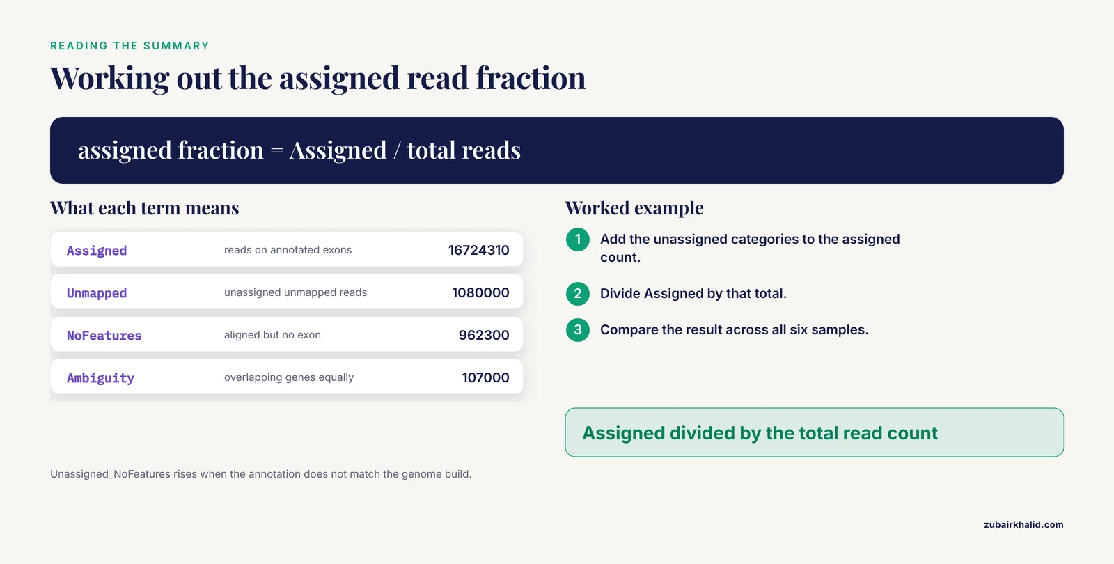
Assigned	16724310
Unassigned_Unmapped	1080000
Unassigned_Read_Type	11200
Unassigned_Singleton	228900
Unassigned_MappingQuality	0
Unassigned_Chimera	0
Unassigned_NoFeatures	962300
Unassigned_Ambiguity	107000

Assigned divided by the total gives the fraction of reads that landed on annotated exons. Unassigned_NoFeatures counts reads that aligned to the genome but not to any annotated exon, which rises when your annotation file does not match your genome build. Unassigned_Ambiguity counts reads that overlap genes equally well, common in dense bacterial genomes and with overlapping eukaryotic genes.

Step 7. Merge Counts into One Matrix

featureCounts writes one file per sample. Differential expression needs all samples as columns of one table. featureCounts can produce that directly if you pass all BAM files to a single call, and a second small script at the project level does exactly that. Save it as scripts/merge_counts.sh:

#!/usr/bin/env bash
set -euo pipefail

PROJECT_DIR="$HOME/rnaseq_tutorial"
COUNT_DIR="$PROJECT_DIR/results/counts"
THREADS=8

mapfile -t BAM_FILES < <(ls "$PROJECT_DIR"/results/aligned/*.sorted.bam)

featureCounts \
    -a "$PROJECT_DIR/reference/genes.gff" \
    -o "$COUNT_DIR/gene_counts_matrix.txt" \
    -T "$THREADS" \
    -p \
    -t exon \
    -g gene_id \
    -s 0 \
    "${BAM_FILES[@]}"

Running it writes a matrix whose first columns are the gene identifiers and whose remaining columns are one per BAM file. Keep the per-sample counts from the main script if you want them for QC. The merged matrix is what feeds DESeq2. If you add samples later, rerun this merge so the matrix includes everyone, then rerun the differential expression step.

Step 8. Run Differential Expression with DESeq2

DESeq2 estimates differential expression from raw counts using a negative binomial model and controls the false discovery rate across all genes. It is installed in its own R environment:

conda create -n rnaseq_r -c conda-forge -c bioconda r-base=4.4 bioconductor-deseq2
conda activate rnaseq_r

Save the following as scripts/run_deseq2.R. It expects an experimental design where sample names contain the group, such as WT_rep1 and KO_rep1, and it compares the second group against the first alphabetically, which here means KO versus WT.

library(DESeq2)

count.file <- file.path(Sys.getenv("HOME"), "rnaseq_tutorial",
                        "results", "counts", "gene_counts_matrix.txt")

raw <- read.delim(count.file, row.names = 1, check.names = FALSE)
counts <- raw[, 6:ncol(raw)]        # drop the annotation columns featureCounts prepends

samples <- data.frame(
    row.names = colnames(counts),
    group = sub("_rep[0-9]+$", "", colnames(counts))
)

samples$group <- factor(samples$group, levels = c("WT", "KO"))

dds <- DESeqDataSetFromMatrix(
    countData = round(counts),
    colData   = samples,
    design    = ~ group
)

dds <- dds[rowSums(counts(dds) >= 10) >= 3, ]   # keep genes with at least 10 counts in 3 samples
dds <- DESeq(dds)

res <- as.data.frame(results(dds, contrast = c("group", "KO", "WT")))
res$gene <- rownames(res)
res <- res[order(res$padj), ]

out <- file.path(dirname(count.file), "deseq2_KO_vs_WT.txt")
write.csv(res, out, row.names = FALSE)

cat("Genes tested:", nrow(res), "\n")
cat("Genes with padj < 0.05 and |log2FC| > 1:",
    sum(res$padj < 0.05 & abs(res$log2FoldChange) > 1, na.rm = TRUE), "\n")
cat("Results written to:", out, "\n")

Run it:

Rscript scripts/run_deseq2.R

Expected output:

Genes tested: 6214
Genes with padj < 0.05 and |log2FC| > 1: 342
Results written to: /home/you/rnaseq_tutorial/results/counts/deseq2_KO_vs_WT.txt

Three design choices in this script deserve explanation. The round() call exists because DESeq2 requires integer counts and some annotation sources produce fractional assignments. The prefiltering line, keeping genes with at least 10 counts in at least 3 samples, is the standard DESeq2 recommendation for reducing the multiple-testing burden on genes too sparse to test. The contrast argument fixes the direction of the comparison so the log2 fold change is KO relative to WT regardless of alphabetical accident.

Step 9. Verify the Results Are Right

Never trust a pipeline you have not checked. Three checks take ten minutes and catch most problems.

Check the QC aggregate. Open results/multiqc/multiqc_report.html in a browser. Every sample should appear. Compare per-sample duplication rates, per-base quality curves, and the fastp trimming summary. One sample that looks unlike the others at this stage will usually look unlike the others in the count table too.

Check alignment consistency. Print the overall alignment rate for all samples from the HISAT2 logs:

grep "overall alignment rate" logs/*_hisat2.log

Expected output:

logs/KO_rep1_hisat2.log:91.42% overall alignment rate
logs/KO_rep2_hisat2.log:90.87% overall alignment rate
logs/KO_rep3_hisat2.log:92.03% overall alignment rate
logs/WT_rep1_hisat2.log:92.10% overall alignment rate
logs/WT_rep2_hisat2.log:91.66% overall alignment rate
logs/WT_rep3_hisat2.log:91.95% overall alignment rate

Samples from the same experiment should land within a few percentage points of each other. A single low outlier usually means a bad library, a wrong adapter setting, or contamination.

Check library-level clustering. Add a variance-stabilized PCA plot to the R script before the results table is written:

vsd <- vst(dds, nsub = 1000)
plotPCA(vsd, intgroup = "group")

Biological replicates from the same condition should cluster together on the first two principal components. If a WT replicate sits with the KO group, you most likely have a sample sheet error, a swapped FASTQ pair, or a genuine outlier. Any of the three must be resolved before you interpret the differential expression table.

Common Errors, Their Exact Messages, and Fixes

hisat2: index does not exist or (ERR): hisat2-build exited with exit status 1. The path in HISAT2_INDEX does not point to the prefix you built, or the build failed partway. Run ls reference/genome_index*.ht2 | wc -l and confirm the answer is 8. If it is, check the variable for typos. If it is not, rerun hisat2-build.

samtools sort: failed to read header from - or a truncated BAM warning. The SAM file from HISAT2 is empty or incomplete, almost always because HISAT2 itself failed. Read logs/<sample>_hisat2.log first. The real error is upstream.

fastp: failed to open file with a path in the message. A sample in samples.csv has no matching FASTQ pair. The script's own preflight check catches this before fastp runs and prints ERROR: missing FASTQ for <sample>. Add the files or remove the sample from the sheet.

The process is killed partway through alignment. Killed in the log, or the script simply dies with no message, means the Linux out-of-memory killer terminated HISAT2. HISAT2 memory use scales with genome size. Yeast fits comfortably in a few gigabytes. Human and mouse indexes need roughly 8 GB per alignment process, so with 8 threads on a 16 GB machine you will be killed. Reduce THREADS to 4, or run on a machine with more RAM.

featureCounts: cannot open file <gtf> or a count matrix of almost all zeros. The annotation does not match the genome build, or the feature type and attribute do not exist in your file. Check what your annotation actually contains:

grep -v "^#" reference/genes.gff | cut -f 3 | sort -u

If this prints gene and CDS but no exon, change -t exon to -t CDS, or convert the annotation to GTF with a tool such as AGAT. Then confirm that the attribute you pass to -g appears in column 9 of the file:

grep -v "^#" reference/genes.gff | head -5

conda: command not found inside the script. The script inherits your shell's PATH only if conda is initialized there. Add source ~/miniconda3/etc/profile.d/conda.sh and conda activate rnaseq at the top of the script, or run the script from within an activated environment.

command not found for any tool despite activation. You activated the wrong environment, or the tool's conda package installed a binary with a different name. Run conda list -n rnaseq | grep fastp to confirm the package and use which fastp to see where the binary lives.

Duplicate sample IDs in the sample sheet. The script will process the sample twice and the second run will overwrite the first outputs. The MultiQC report will show two entries for the same sample name. Always keep sample IDs unique.

Common Mistakes and Limitations

Mistracking strandedness. The -s flag of featureCounts is the most consequential single parameter in the counting step, and it is the one most often left at its default without thought. An unstranded library counted as stranded, or the reverse, can roughly halve the reads assigned to genes and distort fold changes. Determine strandedness from your library kit documentation, or empirically with a tool such as RSeQC, and set STRANDEDNESS accordingly.

Mixing genome builds. The HISAT2 index and the annotation file must come from the same genome release. Aligning to one build while counting against another inflates Unassigned_NoFeatures and can silently assign reads to coordinates that no longer exist. Download both files from the same source release, in the same session, into the same folder.

Treating the script as validation. A script that runs to completion is not the same as an analysis that is correct. The script guarantees that commands executed in order. It does not guarantee that your sample sheet is right, that your groups are balanced, or that your biological question matches the design formula. The PCA and alignment-rate checks in Step 9 are the part of the workflow that catches those problems, and they require a human to look at the output.

Confusing bash automation with workflow management. Bash runs samples one after another and stops at the first failure. It does not skip samples that already finished on a rerun, it does not submit parallel jobs to a scheduler, and it does not resume from the failed step. For a one-project, six-sample analysis that is fine. Published pipelines in this space offer two implementation options, one in bash with SLURM and one in Nextflow, precisely because straightforward bash is easy to install and modify while workflow managers handle resumption, parallelism, and portability across computing environments [1]. When your sample count grows or you move to a cluster, treat the bash script as the specification and port it.

Forgetting that reproducibility includes software versions. The script records what you ran, but the environment matters as much as the commands. The reproducibility gains described for automated pipelines assume a pinned software environment [2]. Export your conda environment with conda env export -n rnaseq > environment.yml, commit both files to the same repository, and note the genome build and annotation release in the project README.

Overwriting raw data. The pipeline never writes into raw_data/, and your script should keep it that way. Trimmed files land in results/trimmed, alignments in results/aligned. If you ever find yourself trimming into the raw folder, stop and fix the paths. Raw FASTQ files are the irreplaceable part of the analysis.

Extending the Script: Parallel Samples and Cluster Execution

The loop processes samples sequentially, which is the safest design but not the fastest. On a machine with enough cores you can run each sample in the background and wait for all of them:

for SAMPLE in "${SAMPLES[@]}"; do
    run_one_sample "$SAMPLE" &
done
wait

To make this work, move the loop body into a function named run_one_sample and give each sample its own log file, as the template already does. Cap the number of concurrent jobs with a simple counter so eight samples do not launch sixteen HISAT2 processes on an eight-core machine:

MAX_JOBS=2
active=0
for SAMPLE in "${SAMPLES[@]}"; do
    run_one_sample "$SAMPLE" &
    active=$((active + 1))
    if (( active >= MAX_JOBS )); then
        wait -n
        active=$((active - 1))
    fi
done
wait

On a cluster using SLURM, the same script becomes a job array. Each array task processes one sample, which is the model used by the bash and SLURM implementation of published RNA-Seq pipelines [1]. The minimal adaptation is a header at the top of a per-sample wrapper:

#SBATCH --job-name=rnaseq
#SBATCH --array=0-5
#SBATCH --cpus-per-task=8
#SBATCH --mem=16G
#SBATCH --time=4:00:00

The array task reads its own sample ID from line SLURM_ARRAY_TASK_ID + 1 of samples.csv and runs the same per-sample chain. Merge counts in a second, separate job after the array completes. The exact scheduler directives vary by institution, so copy the header format from your cluster's own documentation rather than from any generic template.

Where to Go Next

The pipeline you have now covers the standard bulk RNA-Seq chain from raw reads to a differential expression table [1]. The productive next steps, in order of value, are these. First, add a batch-effect check by including a batch column in the DESeq2 design formula if your samples were prepared on more than one day. Second, keep a per-project conda environment.yml and the samples.csv in version control alongside the scripts. Third, when the project outgrows one script, port the same steps to Nextflow or Snakemake, keeping the tool versions and parameters identical so results stay comparable. The effort you spent making the bash script explicit is exactly what makes that port mechanical, because every choice is already written down.

Frequently Asked Questions

Can a bash script really handle a complete RNA-Seq analysis?

Yes, for a straightforward bulk RNA-Seq project a single bash script can run quality control, trimming, alignment, and counting end to end, and published pipelines offer a bash implementation alongside more complex workflow-manager options [1]. What bash cannot do on its own is parallel scheduling, automatic resumption of failed steps, and software containerization, which is where Nextflow or Snakemake earn their keep.

How many samples can I process with one bash script?

Dozens, because the loop simply repeats per sample. The practical constraint is runtime and memory, not the script. If you find yourself running the script repeatedly after failures, or wanting samples to process simultaneously on a cluster, that is the signal to move to a workflow manager or a SLURM job array.

Do I need root or administrator access?

No. Conda installs entirely in your home directory, all pipeline outputs live in your project folder, and none of the commands in this article touch system paths. This is the normal situation on shared university clusters.

What changes for single-end data?

Three things. Drop the -2 argument from HISAT2 and the -I and -O arguments from fastp, remove the paired-end flag -p from featureCounts, and name FASTQ files without the _1 and _2 suffixes. Everything else in the script stays the same.

Which reference genome should I use?

Use the genome build and annotation release that match your organism and your experimental design, downloaded together from the same source. For quick testing, a small genome such as yeast aligns in minutes. The critical rule is that the HISAT2 index, the annotation file, and the genome build must all agree.

Why is my alignment rate much lower than my collaborator's?

The most common causes are mismatched genome builds, wrong adapter or strandedness settings, the wrong organism reference, and genuinely poor library quality in that order. Compare the fastp report and the HISAT2 log for the weak sample against a good one, and check that both of you used the same reference release.

How do I add new samples to an existing analysis?

Append the new sample IDs to samples.csv, drop their FASTQ files into raw_data/, and rerun both scripts. The per-sample steps are idempotent, and the merged count matrix is regenerated from all BAM files, so the differential expression analysis automatically includes the new samples.

Where do I look first when the script fails?

Read the last lines of logs/ for the sample that was being processed when it stopped. The timestamped log lines tell you which step was running, the tool-specific log file contains the actual error, and set -euo pipefail guarantees the script stopped at the true point of failure rather than continuing past it.

Sources

1. RNA-SeqEZPZ: A Point-and-Click Pipeline for Comprehensive Transcriptomics Analysis with Interactive Visualizations.
2. admixr-R package for reproducible analyses using ADMIXTOOLS.