Automating Data Quality Control in Genomics: Scripts and Workflows

By Dr. Zubair Khalid, DVM, MS, PhD · 2026-11-11

By the end of this guide you will be able to build a quality control (QC) layer that runs unattended on new sequencing or genotyping data. You will install a QC toolchain with one command, run raw-read and post-alignment checks, trim adapters, compute per-sample coverage, apply standard genotyping filters, wrap everything in a logged shell script, and hand the whole workflow to a workflow manager so it reruns the same way every time. You will also know which metrics deserve automated thresholds, which errors you will hit on the first run, and how to store and report the results so they survive an audit or a publication review.

To follow along you need a Linux or macOS machine (or a Slurm or cloud batch environment), at least 16 GB of RAM for the examples shown, 50 GB of free disk for a small test dataset, and the Conda or Micromamba package manager. Every command in this guide runs on data you can generate or substitute with your own FASTQ and BAM files.

Quality control is the groundwork of any sequencing analysis pipeline. RNA-seq analysis guides place QC first for exactly this reason, because every downstream count, fold change, and pathway call inherits whatever problems the raw data carry [1]. Genome-wide association study (GWAS) practice makes the same point from the array side, with an explicit emphasis on automating data storage, filtering, and manipulation so data integrity holds through the whole process [2]. The pattern generalizes across genomics. Once datasets reach the scale of modern high-throughput studies, manual QC becomes the bottleneck and the error source, which is why recent reviews of data stewardship in AI-based genomics treat quality management, traceability, and automated curation as first-class infrastructure rather than optional extras [3].

What Automated QC Means in Practice

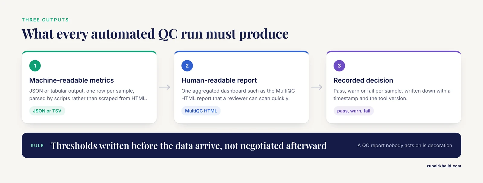
Three-step flow showing the metrics file, the aggregated HTML report and the recorded pass, warn or fail decision each QC run must leave behind.

Manual QC means a person opens per-sample reports, eyeballs them, and decides whether to proceed. Automated QC means the same checks run by script, against thresholds written down in advance, with three artifacts produced every time:

Machine-readable metrics, such as JSON or tabular output, one row per sample.
A human-readable report, such as an aggregated HTML dashboard, that a reviewer can scan quickly.
A pass, warn, or fail decision per sample, recorded with a timestamp and tool version.

That third artifact is the piece people skip. A QC report nobody acts on is decoration. Decisions can be soft (flag the sample, email the lab) or hard (drop the sample from the run), but they must be written down before the data arrive, not negotiated afterward. Standardized, documented QC is what makes datasets comparable across batches and shareable for combined analysis, a point biobanking workflow research has emphasized for years [4].

The payoff for doing this well is measurable. In a large study of optical coherence tomography volumes from the UK Biobank, an automated QC tool that scored volumetric misalignment before biomarker extraction increased significant genetic associations by 21.1 percent and heritability estimates by 19.1 percent compared with less rigorous screening [5]. The modality differs from short-read sequencing, but the lesson transfers directly: automated QC at the front of the pipeline changes the statistics at the end of it.

The Toolchain at a Glance

The commands below use a small, stable set of open-source tools available through Bioconda. You do not need all of them on day one. The first four cover most sequencing workflows.

Tool	Job	Output you keep
FastQC	Per-file raw read metrics	HTML plus zip per FASTQ
fastp	Adapter and quality trimming with QC metrics	Trimmed FASTQ, JSON and HTML report
samtools	Alignment-level QC	flagstat, idxstats, stats text files
mosdepth	Per-base and per-region coverage	Per-base depth, summary TSV
MultiQC	Aggregates all tool outputs into one dashboard	One HTML report per run
PLINK 2	Genotype array filtering	Filtered BED/BIM/FAM plus log
Nextflow	Workflow orchestration and resuming	Execution log, cache, reports
picard	Alignment metrics, duplicate marking, validation	Metrics tables

Automate Genomics Data QC Step by Step

This walkthrough uses paired-end Illumina data. Adapt file names to your own run. Each step shows the command, the parameters that matter, and what correct output looks like.

Step 1: Set Up a Reproducible Environment

Create a dedicated environment so tool versions are pinned and reinstallable. Version drift between runs is one of the quietest ways QC numbers become incomparable across months.

mamba create -n gqc -c conda-forge -c bioconda \
  fastqc=0.12.1 multiqc=1.21 fastp=0.23.4 \
  samtools=1.19.2 mosdepth=0.3.8 bwa-mem2=2.2.1 \
  plink2 picard
mamba activate gqc

Check the environment resolves before you trust it.

fastqc --version
# 0.12.1
multiqc --version
# multiqc, version 1.21
samtools --version | head -n 1
# samtools 1.19.2

Pin the exact versions in a YAML file checked into version control. When a collaborator gets different numbers from the same FASTQ files six months from now, the environment file is usually the first suspect and the first thing you can rule out.

Step 2: Compute Checksums Before Anything Touches the Data

QC on files that were corrupted during transfer is wasted work. Record checksums at ingestion and verify them before every run.

md5sum data/*.fastq.gz > data/md5.txt
md5sum -c data/md5.txt
# data/sample_A_R1.fastq.gz: OK
# data/sample_A_R2.fastq.gz: OK

A failed line reads FAILED open or read followed by a nonzero exit code. That failure means re-transfer the file, not analyze it anyway.

Step 3: Run Raw-Read QC

FastQC computes per-base quality scores, adapter content, GC distribution, duplication levels, overrepresented sequences, and sequence length distributions, one report per FASTQ file.

mkdir -p qc/fastqc_raw
fastqc -t 8 -o qc/fastqc_raw \
  data/sample_A_R1.fastq.gz data/sample_A_R2.fastq.gz

Parameters that matter:

-t 8 sets threads. FastQC parallelizes across input files, so this scales with how many files you pass in one call.
-o sets the output directory. Without it, reports land in the current directory and pollute your project root.
Input files accept a glob such as data/*.fastq.gz, which is what you want in an automated loop.

Correct output per file pair is a pair of files:

qc/fastqc_raw/sample_A_R1_fastqc.html
qc/fastqc_raw/sample_A_R1_fastqc.zip
qc/fastqc_raw/sample_A_R2_fastqc.html
qc/fastqc_raw/sample_A_R2_fastqc.zip

Inside the HTML, the numbers to automate decisions on are the per-base sequence quality boxplots (watch for the tail dropping below Q20, meaning a 1 percent error probability), adapter contamination percentages, per-base sequence content imbalance in the first dozen cycles, and overrepresented sequences. Individual samples vary. The value of automation is that you compare every sample against the same written thresholds rather than against your mood that morning.

Step 4: Trim Adapters and Low-Quality Tails

fastp performs trimming and emits its own machine-readable metrics in the same run, which removes the need for a separate trimming QC step.

mkdir -p trimmed qc/fastp
fastp \
  -i data/sample_A_R1.fastq.gz \
  -I data/sample_A_R2.fastq.gz \
  -o trimmed/sample_A_R1.trim.fastq.gz \
  -O trimmed/sample_A_R2.trim.fastq.gz \
  --detect_adapter_for_pe \
  --qualified_quality_phred 20 \
  --length_required 50 \
  --thread 8 \
  --html qc/fastp/sample_A.html \
  --json qc/fastp/sample_A.json \
  2> qc/fastp/sample_A.log

Parameter by parameter:

-detect_adapter_for_pe enables adapter detection for paired-end data by overlap analysis, useful when the library preparation protocol is unknown or variable.
-qualified_quality_phred 20 keeps bases at Phred quality 20 or above for the main filtering pass. Phred 20 corresponds to a 1 percent base-call error probability.
-length_required 50 discards reads shorter than 50 bases after trimming, which keeps fragments that remain useful for alignment while dropping slivers.
-json output is the artifact your automation reads. Parse it with jq in the next step.

A trimmed JSON report contains before and after summaries. Two fields worth extracting automatically:

jq '.summary.before_filtering.total_reads, .summary.after_filtering.total_reads' \
  qc/fastp/sample_A.json
# 24000000
# 23558411

A retention rate below roughly 90 percent of raw reads is a conventional warn-level signal that the library had heavy adapter or quality problems. Investigate the run, not just the sample.

Step 5: Align and Run Post-Alignment QC

Alignment itself is not QC, but the alignment metrics are. A minimal pattern:

mkdir -p bam qc/flagstat
bwa-mem2 mem -t 16 ref/hg38.fa \
  trimmed/sample_A_R1.trim.fastq.gz trimmed/sample_A_R2.trim.fastq.gz \
  | samtools sort -@ 8 -o bam/sample_A.bam -
samtools index bam/sample_A.bam
samtools flagstat -@ 8 bam/sample_A.bam > qc/flagstat/sample_A.txt

Correct flagstat output looks like this (numbers will differ):

23558411 + 0 in total (QC-passed reads + QC-failed reads)
47116822 + 0 primary
46989900 + 0 mapped (99.73% : N/A)
46989900 + 0 primary mapped (99.73% : N/A)

The two percentages you gate on are the primary mapped percentage and the properly paired percentage that appears further down the report. For human whole-genome or whole-exome data on a correct reference build, primary mapped rates below the mid-90s in percent usually mean sample contamination, wrong reference build, or heavily degraded input. Treat a sample that maps poorly as a lab problem to escalate, not a numbers problem to tune around.

Depth per target region matters for exomes and panels. mosdepth gives it in one pass:

mosdepth --threads 8 --by targets.bed qc/mosdepth/sample_A bam/sample_A.bam
cat qc/mosdepth/sample_A.mosdepth.summary.txt
# chrom  length  mean  min  max
# total  3209286290  31.42  0  380

The mean column answers the question reviewers always ask about exomes: what was the mean on-target depth.

Step 6: Genotype Array QC With Written-Down Filters

Array data need a different filter set, and the standard metrics are call rate per sample and per variant, minor allele frequency, heterozygosity outliers, sex concordance, relatedness, and Hardy-Weinberg equilibrium deviations. A GWAS-oriented QC chapter walks through exactly this progression from raw data to a fully filtered dataset, with automation of storage and filtering emphasized throughout [2]. Dedicated automated pipelines formalize it. SNPQC applies user-defined thresholds across common quality metrics, writes a QC report, and stores genotypic, phenotypic, and quality metrics in a database so later runs can be integrated with the same integrity guarantees [6]. GTQC automates the same territory as an R package and produces a detailed HTML report across a broad set of metrics [7].

A compact PLINK 2 pass using widely used defaults:

plink2 \
  --bfile raw/sample_batch \
  --geno 0.02 --mind 0.02 \
  --maf 0.01 --hwe 1e-6 midp \
  --make-bed --out filtered/sample_batch

-geno 0.02 drops variants missing in more than 2 percent of samples.
-mind 0.02 drops samples missing more than 2 percent of genotypes.
-maf 0.01 drops variants below 1 percent minor allele frequency.
-hwe 1e-6 midp drops variants with exact-test equilibrium departure below the threshold on control samples, using the mid-p adjustment that reduces over-filtering of rare variants.

The PLINK log reports how many samples and variants each filter removed. Save every log. A filtered dataset whose log does not state its starting counts is unverifiable, and downstream users will treat it accordingly.

Population stratification deserves its own automated step, and it is the kind of step that benefits from being a pipeline module rather than an ad hoc notebook. The snpQT pipeline, built on Nextflow and BioContainers, implements around 36 discrete quality filters or correction steps including genome build conversion, population stratification against 1000 Genomes reference data, automated population outlier removal, and imputation with pre- and post-imputation QC, all producing graphical before-and-after reports [8]. If your project is human genotyping at any real scale, look at that architecture before writing your own.

Step 7: Wrap It All in a Logged, Fail-Fast Script

The script is where automation becomes real. Three properties matter: it stops on the first failure, it timestamps every stage, and it emits one aggregated report at the end.

#!/usr/bin/env bash
set -euo pipefail

SAMPLES="sample_A sample_B sample_C"
THREADS=8
OUT=qc
mkdir -p trimmed qc/fastqc_raw qc/fastp qc/flagstat qc/multiqc

for S in ${SAMPLES}; do
  echo "[$(date -Is)] START raw QC ${S}" | tee -a qc/run.log
  fastqc -t ${THREADS} -o ${OUT}/fastqc_raw \
    data/${S}_R1.fastq.gz data/${S}_R2.fastq.gz

  echo "[$(date -Is)] START trim ${S}" | tee -a qc/run.log
  fastp \
    -i data/${S}_R1.fastq.gz -I data/${S}_R2.fastq.gz \
    -o trimmed/${S}_R1.trim.fastq.gz -O trimmed/${S}_R2.trim.fastq.gz \
    --detect_adapter_for_pe --qualified_quality_phred 20 \
    --length_required 50 --thread ${THREADS} \
    --html ${OUT}/fastp/${S}.html --json ${OUT}/fastp/${S}.json \
    2> ${OUT}/fastp/${S}.log

  echo "[$(date -Is)] START align ${S}" | tee -a qc/run.log
  bwa-mem2 mem -t 16 ref/hg38.fa \
    trimmed/${S}_R1.trim.fastq.gz trimmed/${S}_R2.trim.fastq.gz \
    | samtools sort -@ 8 -o bam/${S}.bam -
  samtools index bam/${S}.bam
  samtools flagstat -@ 8 bam/${S}.bam > ${OUT}/flagstat/${S}.txt

  echo "[$(date -Is)] DONE ${S}" | tee -a qc/run.log
done

multiqc ${OUT} -o ${OUT}/multiqc -n run_summary
echo "[$(date -Is)] MultiQC report written" | tee -a qc/run.log

Line-by-line, the parts that prevent 2 a.m. failures:

set -euo pipefail exits on any nonzero command, on any unset variable, and on any failure inside a pipeline. Without pipefail, a silent bwa-mem2 crash still lets samtools finish on empty input and the run looks successful.
tee -a qc/run.log gives you one timestamped run log you can grep months later.
The trailing - on samtools sort tells it to read from standard input, which is how the alignment pipe stays a pipe.

Expected ending output:

[2026-11-11T09:14:02-05:00] START raw QC sample_A
[2026-11-11T09:31:47-05:00] START trim sample_A
[2026-11-11T09:44:10-05:00] START align sample_A
[2026-11-11T10:02:55-05:00] DONE sample_A
[2026-11-11T10:07:18-05:00] MultiQC report written

Step 8: Aggregate Everything With MultiQC

MultiQC parses FastQC, fastp, samtools stats, mosdepth, and dozens of other tool outputs into one dashboard.

multiqc qc/ -o qc/multiqc -n run_summary

Correct behavior on a three-sample run prints a summary similar to:

[INFO]         multiqc : This is MultiQC v1.21
[INFO]           fastqc : Found 6 reports
[INFO]            fastp : Found 3 reports
[INFO]         mosdepth : Found 3 reports
[INFO]   MultiQC complete | qc/multiqc/run_summary.html

The dashboard is the artifact you archive with the run. It is also where small per-sample anomalies jump out that per-sample files hide, for example one library with an adapter profile unlike its batchmates.

Step 9: Hand the Workflow to Nextflow

A shell loop reruns everything from scratch every time. A workflow manager caches completed steps, parallelizes correctly, and documents dependencies. Nextflow is the pattern behind snpQT, which pairs it with BioContainers so the same pipeline runs on laptops, HPC clusters, and cloud instances with the same behavior [8].

A minimal process shows the shape:

process TRIM {
  tag "${sampleId}"
  input:
  tuple val(sampleId), path(read1), path(read2)
  output:
  tuple val(sampleId), path("*_R1.trim.fastq.gz"), emit: r1
  tuple val(sampleId), path("*_R2.trim.fastq.gz"), emit: r2
  path "*fastp.json", emit: json
  script:
  """
  fastp -i ${read1} -I ${read2} \
    -o ${sampleId}_R1.trim.fastq.gz \
    -O ${sampleId}_R2.trim.fastq.gz \
    --detect_adapter_for_pe --length_required 50 \
    --json ${sampleId}.json
  """
}

With -with-report -with-trace -resume on the command line, Nextflow gives you a cached, resumable, resource-tracked run. The first investment is a day. The return shows up the first time a 40-sample run dies at sample 38 and resumes in minutes.

Genomics Data Storage and Bioinformatics Data Management

QC automation is inseparable from storage design, because QC outputs are data too, and because the decision of whether to keep a sample must be traceable to the original files months or years later. Reviews of data stewardship in AI-driven genomics group the requirements explicitly: data governance, quality management, privacy measures, access control, accountability, traceability, curation frameworks, and storage systems [3]. Four practices cover the storage side for most labs.

First, separate tiers. Raw FASTQ and BAM files are immutable and belong on cheap, large storage or object storage. QC metrics, logs, and reports are small and belong somewhere queryable, which is why SNPQC writes quality metrics into a database rather than scattering text files, specifically to maintain integrity across subsequent genotyping runs [6].

Second, name files so scripts never have to guess. A convention such as {study}_{sampleId}_{library}_{lane}_{R1|R2}.fastq.gz lets your QC script derive sample identity from the file name and prevents the merge-ups that manual renaming produces.

Third, record access conditions in machine-readable form alongside the data. The GA4GH Data Use Ontology encodes a dataset's allowable uses as structured terms, is implemented by major institutes, and annotates well over 200,000 datasets worldwide, which means automated pipelines can check permissions rather than relying on memory or emails [9].

Fourth, keep sample identity provable. The PGP-UK reference panel implemented genotype-based validation specifically to exclude sample mix-ups across its genomic, methylomic, and transcriptomic data [10]. An automated identity check, even a simple cross-platform SNP concordance test between sequencing and array data, catches the single most damaging class of error a QC program can face.

For projects that combine molecular data with clinical records, data model harmonization matters as much as file storage. The All Of Us program standardized EHR data around the OMOP common data model, and pipeline work transforming i2b2 warehouse data into OMOP shows how ontology-driven transformation avoids site-specific programming [11]. If your QC outputs will ever meet an EHR-derived phenotype table, plan the identifier mapping before the first run, not after the first discordant result.

Long-lived repositories demonstrate the endpoint of this discipline. NCRAD has banked biospecimens and linked data from 91 studies and over 135,000 participants, distributing over 440,000 aliquots, sustained by documented best practices for collection, processing, and distribution [12]. The biobanking literature behind such repositories stresses that QC of the sample itself, documented and validated, is what establishes context for interpreting every downstream result [4]. A QC pipeline that archives its evidence, thresholds, and decisions per sample is doing the digital equivalent of what those repositories do physically.

Reporting, Provenance, and Submission-Ready QC

Automated QC reports should serve three audiences at once. The bench scientist needs today's run summarized. The collaborator needs last quarter's batch compared against this one. The reviewer or regulator needs proof of what was checked, with what tool, at what version.

Integrated platforms solve this by storing QC alongside analysis results and provenance. The Ludmer Centre's work consolidating heterogeneous genetic and epigenetic datasets into the LORIS platform, with results linked to provenance information and pipelines shared in versioned form through the CBRAIN processing portal, is a concrete example of that pattern at institutional scale [13]. You do not need their infrastructure to copy the principle. Keep, per run, the tool versions, the exact command lines, the thresholds in force, and the git commit of the pipeline itself.

For data headed to public archives, QC and submission are one workflow. The GenomeTrakr-oriented protocols for enteric pathogen genomic surveillance define a standard data package with separate protocols for QC assessment of sequence data, validation of contextual metadata, submission to an INSDC repository, and ongoing curation, with NCBI Pathogen Detection providing automated cluster analyses on top [14]. The general lesson for any lab is that submission requirements are QC requirements. If the archive will reject a mislabeled sample or an incomplete metadata record, your pipeline should reject it first.

Clinical pipelines raise the bar again. End-to-end clinical NGS analysis implements QC metrics at each pipeline step against a validated training dataset to ensure data integrity for clinical applications [15]. Even if your setting is research, borrowing the habit of validating metrics against a reference dataset gives you a calibration point that pure thresholds lack.

One more automation channel worth knowing: validators built for continuous integration. The mmCIF Validator ships as both an editor extension and a standalone Python script intended for batch processing and integration into automated workflows and CI/CD pipelines, so structural data files are validated on every commit rather than at deposition time [16]. The same CI pattern applies to any QC you can express as a command. A pipeline test that runs your QC script on a small fixture dataset whenever the pipeline code changes catches most regressions before they ever meet real data.

Automate Genomics Data QC Tips That Hold Up at Scale

Write thresholds in a config file, never in the script body. A YAML file with min_q30: 0.85 and max_adapter_pct: 5 turns your QC policy into a versioned, reviewable document.
Parse JSON, never HTML. fastp, mosdepth, and most modern tools emit JSON. Scripts that scrape HTML reports break on every tool update.
Fail loudly, warn quietly. A missing FASTQ should stop the run. One sample with slightly low Q30 should annotate the report and continue.
Compare against batch, not absolutes, for some metrics. GC content and duplication have context-dependent expectations, so an automated z-score against the current batch often beats a fixed cutoff.
Track per-run tool versions automatically by having the script dump -version output for every tool into the run log.
Test your pipeline on a fixture dataset after every code change. Five minutes of CI prevents the failure mode where a renamed column silently empties your summary table for three months.
Keep raw data read-only. Set directory permissions so the QC pipeline can write reports but not touch source FASTQ files.
Validate sample identity programmatically when you have both sequencing and genotype data, following the mix-up-detection practice documented for multi-omics reference panels [10].

Common Mistakes and Limitations

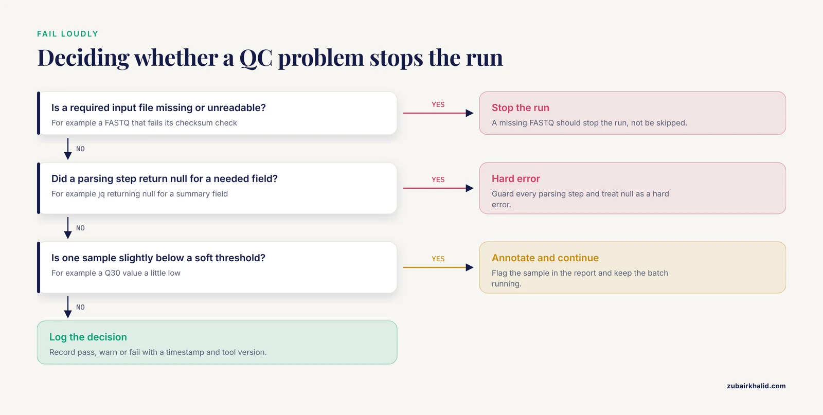
Decision path separating hard failures that stop the run from soft warnings that annotate the report and let the batch continue.

Silent success is the defining failure of automated QC. A script that exits zero while producing empty reports is worse than no script. Guard every parsing step. If jq returns null for a field your summary depends on, that should be a hard error.

Threshold archaeology is the second chronic failure. Teams inherit cutoffs from a pipeline written years ago for a different assay. A mean depth threshold calibrated for a 100 megabase panel is meaningless for whole-genome data. When you adopt a pipeline, document where each threshold came from and re-derive the ones nobody can explain.

Cross-sample contamination is invisible to most per-sample metrics. A diploid human sample with 15 percent foreign DNA can pass quality, depth, and mapping checks while corrupting variant calls. Detection needs a dedicated method such as verifyBamID-style analysis or sex chromosome concordance. Budget for it in human work.

Automation without stewardship creates clean garbage at scale. The governance dimensions that reviews of AI-based genomics emphasize, including privacy, access control, accountability, and traceability, are not automatic side effects of running a pipeline [3]. A pipeline with no access controls, no audit trail, and no consent metadata attached is faster at producing data you may not be permitted to share.

Over-trimming is a real and quantifiable loss. Aggressive adapter and quality filtering throws away bases that alignment would have used. If your trim step removes more than about 10 percent of reads or more than a few bases per read on well-run libraries, suspect overactive defaults rather than bad libraries, and check the fastp before-and-after histogram.

Finally, the structural limitation: automated QC validates what you thought to measure. Expression-based QC in single-cell analysis exists precisely because library-level metrics cannot distinguish true biological variation from background noise, which is why frameworks such as scQCEA add automated cell type annotation as an expression-based quality layer on top of standard metrics [17]. Single-cell libraries have platform-specific behavior, and shallow-sequenced profiles have their own quality distributions, so thresholds transfer poorly across platforms. Treat every threshold as platform-local evidence, and expect to recalibrate when the instrument, chemistry, or reference changes.

Frequently Asked Questions

What does automating data quality control in genomics actually involve?

It means running the same QC checks on every sample with scripts, against thresholds written in advance, and producing machine-readable metrics, a human-readable report, and a recorded pass or fail decision each time. The automation replaces manual inspection, not the judgment about what good data look like.

Which tools should I start with for automated genomics QC?

Start with FastQC for raw reads, fastp for trimming with built-in metrics, samtools flagstat for alignment, and MultiQC to aggregate all reports into one dashboard. Those four cover most short-read sequencing projects and install together from Bioconda in a single environment.

Can I automate genomics data QC step by step without coding experience?

You can get surprisingly far with a single shell script and a workflow manager because mature pipelines such as snpQT wrap dozens of QC steps behind a command-line interface with minimal coding required [8]. Start by running established pipelines rather than writing your own, and learn the config files before you learn the code.

How do I choose QC thresholds so they are defensible?

Anchor every threshold to something citable: a tool's documented default, a published pipeline, or your own batch history. For genotype arrays, call rate, MAF, and Hardy-Weinberg filters have well-established conventional values in the GWAS QC literature [2]. For sequencing metrics, calibrate against your instrument and platform, and record the evidence in the config file itself.

What are the most common mistakes in automating genomics data QC?

Silent failures that still exit zero, thresholds inherited without re-derivation, HTML scraping instead of JSON parsing, ignoring cross-sample contamination, and archiving reports without tool versions or pipeline provenance. Each one produces a pipeline that looks healthy while degrading the science.

How much genomics data storage do I need and how should I organize it?

Plan for tiers rather than a single number: immutable raw files on bulk storage, aligned intermediates on faster storage, and small QC metrics in a queryable database. The stewardship literature treats storage systems, traceability, and curation as connected design problems rather than a capacity question alone [3].

Should QC results be submitted to public repositories along with the data?

Submission packages for public archives include QC assessment and validated contextual metadata as distinct protocol steps, so QC evidence travels with the data by design [14]. Keeping your internal QC artifacts submission-shaped from the start makes public deposit a rerun rather than a rescue project.

How often should QC be re-run on archived data?

Re-run QC whenever the raw files move, whenever the pipeline or tool versions change, and whenever a new downstream analysis will consume stored data for the first time. Verifying checksums before reuse catches silent corruption, and re-executing the QC layer proves the archived dataset still passes the thresholds it was accepted under.