How to Annotate Genomic Ranges with Gene Symbols in R

By Dr. Zubair Khalid, DVM, MS, PhD · 2026-11-11

By the end of this tutorial you will be able to take any set of genomic intervals, such as ChIP-seq peaks, ATAC-seq peaks, copy-number segments, or GWAS loci, and attach human-readable gene symbols to them in R. You will learn how to load ranges into a GRanges object, harmonize chromosome names and genome builds, choose an overlap rule, convert internal gene identifiers to symbols with Bioconductor annotation databases, and validate the resulting symbols against the HGNC records so that aliases and spreadsheet-corrupted names do not slip into your final table. This is a core skill in r for bioinformatics work, and the whole pipeline runs locally in a single R session.

Before you start, install R (version 4.4 or newer works with current Bioconductor releases) and have roughly 2 GB of free disk space for the annotation databases. The packages you need are GenomicRanges, rtracklayer, GenomeInfoDb, AnnotationDbi, org.Hs.eg.db, a transcript database such as TxDb.Hsapiens.UCSC.hg38.knownGene, and HGNChelper for symbol correction. If you have never worked with a Bioconductor tutorial before, the pattern is always the same: install through BiocManager, load with library(), and query annotation objects with functions from AnnotationDbi.

A note on scope. Every step below works the same way for mouse, rat, or any organism with a Bioconductor annotation package. The examples use human data because that is the most common case, and because human gene nomenclature illustrates the identifier problems you must plan for in any species.

What Gene Symbols Are and Why They Complicate Annotation

A genomic range is a coordinate triple: a chromosome, a start position, and an end position. A gene symbol is a short label like TP53 or CFTR. Turning one into the other sounds like a simple table join, but gene symbols are notoriously unstable identifiers. They accumulate aliases and outdated forms, they are corrupted by spreadsheet software that converts names like SEPT1 into dates, and they change over time as nomenclature committees revise records [1].

The scale of the ambiguity problem is worth internalizing before you write any code. A survey of protein-coding gene nomenclature in the Ensembl genome browser found that the total number of official symbols and synonyms used to label protein-coding genes reaches roughly 64,580 in mouse, and that a large fraction of symbols map to more than one gene. The authors estimated that ambiguous symbols could complicate identification of about 18 percent of human protein-coding genes and about 10 percent of rat and mouse genes, and they recommended using stable identifiers from bodies such as Ensembl, NCBI, and HGNC as the primary key, with symbols as display labels [2]. Established annotation tools built for knowledge-driven filtering treat identifier ambiguity as a first-class problem, which is why systems such as Biofilter expose explicit controls for how ambiguous gene identifiers are handled when annotating genomic locations [3].

The practical consequence for your R workflow is this: use coordinates to find which genes overlap or neighbor your ranges, use stable gene IDs (Entrez Gene IDs or Ensembl gene IDs) as the join key, and only convert to symbols at the last step, after validating them. Coordinates never go stale. Symbols do.

One more piece of historical context explains why coordinate-based annotation is the standard. Early approaches to locating sequence-defined elements in a genome relied on sequence search itself, for example electronic PCR implementations that searched large genomes for sequence-tagged sites and could interpret ranges in their search fields [4]. That approach works but is slow and awkward compared with interval arithmetic on coordinate systems, which is what findOverlaps in GenomicRanges does in milliseconds.

Setup: Installing the Bioconductor Stack

Open R (or RStudio) and run:

install.packages("BiocManager")
BiocManager::install(c(
  "GenomicRanges",
  "GenomeInfoDb",
  "rtracklayer",
  "AnnotationDbi",
  "org.Hs.eg.db",
  "TxDb.Hsapiens.UCSC.hg38.knownGene",
  "EnsDb.Hsapiens.v86",
  "AnnotationHub",
  "ChIPseeker",
  "HGNChelper"
))

The first install takes 15 to 45 minutes depending on your machine because some dependencies compile from source. HGNChelper installs from CRAN and provides symbol checking against the HGNC human and MGI mouse databases, including detection of symbols mangled by spreadsheet software [1].

Check that everything loads:

library(GenomicRanges)
library(GenomeInfoDb)
library(rtracklayer)
library(AnnotationDbi)
library(org.Hs.eg.db)
library(HGNChelper)

packageVersion("GenomicRanges")
packageVersion("org.Hs.eg.db")

Record these version numbers. Annotation databases change between releases, and a colleague reproducing your annotation six months later needs to know exactly which gene model you used.

How to Annotate Genomic Ranges with Gene Symbols, Step by Step

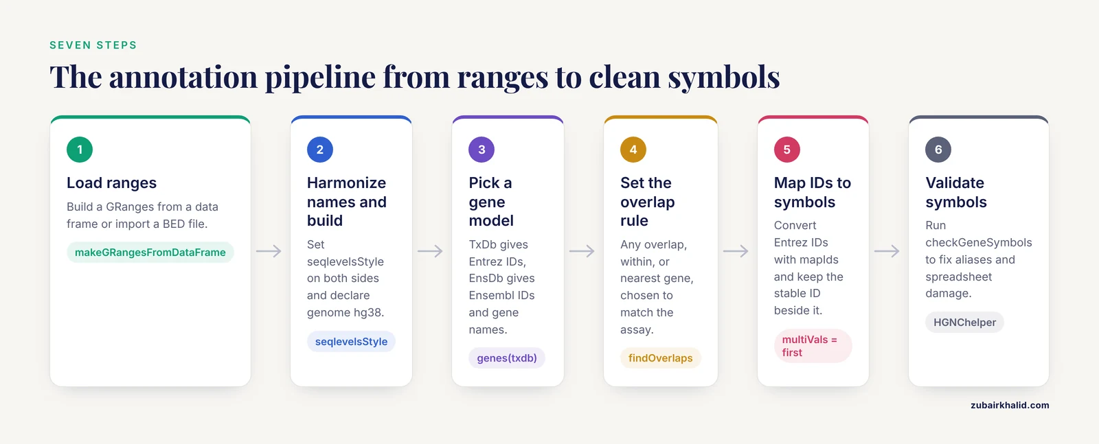
This section is the core walkthrough. Each step builds on the previous one, and the full runnable script appears at the end of the section.

Step 1: Load Your Ranges into a GRanges Object

GRanges is the central data structure in GenomicRanges. It stores chromosome names, intervals, strand, and any metadata columns side by side so that interval operations and metadata stay synchronized.

If your ranges are already in R, for example as a data frame from DESeq2, edgeR, or a peak caller, convert them directly:

library(GenomicRanges)

df <- data.frame(
  chrom  = c("chr1", "chr7", "chr17"),
  start  = c(1200, 2200, 3100),
  end    = c(1400, 2400, 3300),
  name   = c("peakA", "peakB", "peakC")
)

peaks <- makeGRangesFromDataFrame(df, keep.extra.columns = TRUE,
                                  seqnames.field = "chrom",
                                  start.field = "start",
                                  end.field = "end")
peaks

Expected output:

GRanges object with 3 ranges and 1 metadata column:
      seqnames    ranges strand |      name
         <Rle> <IRanges>  <Rle> | <character>
  [1]     chr1   1200-1400      * |     peakA
  [2]     chr7   2200-2400      * |     peakB
  [3]    chr17   3100-3300      * |     peakC
  -------
  seqinfo: 3 sequences from an unspecified genome, no seqlengths

If your ranges live in a BED file, rtracklayer reads them while preserving the score and name columns:

library(rtracklayer)
peaks <- import("peaks.bed", format = "BED")

BED coordinates are zero-based and half-open, while GRanges uses one-based closed intervals. import() performs the conversion for you. If you ever read BED coordinates by hand with read.table, add 1 to the start column before building the GRanges, or your annotations will be shifted by one base.

Step 2: Harmonize Chromosome Names and Genome Build

This step prevents the single most common silent failure in range annotation. Chromosome naming follows two conventions. UCSC uses the prefix chr (chr1, chrX, chrM). Ensembl and NCBI RefSeq use bare numbers (1, X, MT). If your peaks say chr1 and your gene database says 1, every overlap operation returns zero results without any error message.

Check what you have on each side:

head(seqlevels(peaks))

Then force both objects to the same style:

seqlevelsStyle(peaks) <- "UCSC"

If a sequence name matches no known style, you will see the message Could not find a unique style mapping for seqlevels. That usually means your file contains scaffold names (GL000009.2, HSCHRUN_RANDOM_CTG4) that have no UCSC-style equivalent. Deal with these by keeping only standard chromosomes for a first-pass annotation:

peaks <- keepStandardChromosomes(peaks, pruning.mode = "coarse")

Next, declare the genome build. Overlap operations between objects with mismatched genome labels can misbehave quietly, and more importantly, coordinates from hg19 and hg38 are genuinely different points in the genome. Set the label so that downstream checks can catch a mismatch:

genome(peaks) <- "hg38"

If your data are hg19 and your annotation database is hg38, do not proceed. Convert one side to the other first, using rtracklayer::liftOver with a chain file obtained through AnnotationHub or the UCSC download server. Chain conversion is beyond the scope of this walkthrough, but you must not skip it, because a 500-base interval on hg19 chromosome 8 rarely lands on the same locus in hg38.

Step 3: Choose a Gene Model Database

You need an object that describes where genes are. Bioconductor gives you three practical choices.

Option A, a UCSC transcript database. TxDb.Hsapiens.UCSC.hg38.knownGene stores gene, transcript, exon, and coding-segment coordinates for the hg38 build, with Entrez Gene IDs as the gene keys:

library(TxDb.Hsapiens.UCSC.hg38.knownGene)
txdb <- TxDb.Hsapiens.UCSC.hg38.knownGene
gene_gr <- genes(txdb)
gene_gr[1:3]

The genes() accessor returns a GRanges of gene bodies. The gene_id metadata column holds Entrez IDs, which is exactly the key type that org.Hs.eg.db expects.

Option B, an Ensembl gene database. EnsDb.Hsapiens.v86 stores Ensembl gene models and can return gene symbols directly alongside Ensembl IDs:

library(EnsDb.Hsapiens.v86)
edb <- EnsDb.Hsapiens.v86
gene_gr_e <- genes(edb, columns = c("gene_id", "gene_name"))

Option C, AnnotationHub for anything else. If you work with another species or another annotation release, query the hub:

library(AnnotationHub)
ah <- AnnotationHub()
results <- query(ah, c("EnsDb", "Homo sapiens"))
edb2 <- results[[1]]

The choice matters for two reasons. First, the genome build must match your ranges. Second, the ID space must match your mapping plan. UCSC TxDb objects hand you Entrez IDs, Ensembl objects hand you Ensembl IDs. Both work. Do not mix them in the same join.

Step 4: Define the Overlap Rule

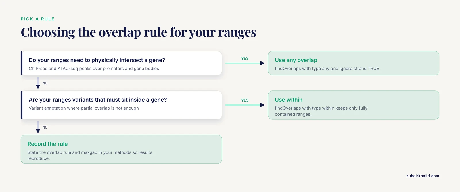
There is no single correct rule for what counts as a hit. The three standard rules are:

1. Any overlap. The range intersects the gene body by at least the minimum overlap width. This is the default and the right choice for ChIP-seq peaks over promoters and gene bodies.
2. Within. The range falls completely inside the gene. Useful for variant annotation.
3. Nearest gene. No overlap required. The range is assigned the closest gene, together with the distance in bases. This is the right rule for intergenic peaks, GWAS lead SNPs, and enhancers.

findOverlaps implements rules 1 and 2, and distanceToNearest implements rule 3. The key parameters are maxgap (the maximum permitted gap, where negative values effectively require an overlap of that depth), minoverlap (the minimum intersecting width under the any rule), and ignore.strand (set TRUE unless your analysis is genuinely strand-specific). Promoter windowing, the convention of extending each gene a fixed distance upstream, is a variant of the nearest rule that you implement with the promoters() helper, shown in Step 5.

Step 5: Find Overlaps and Extract Gene IDs

With peaks and gene bodies on the same naming convention and build, the overlap step is one call:

hits <- findOverlaps(peaks, gene_gr, ignore.strand = TRUE)
hits

The returned Hits object holds paired indices. queryHits(hits) indexes into peaks, subjectHits(hits) indexes into gene_gr. A peak that touches three genes appears three times, which is the correct behavior, and you decide later how to collapse it.

For nearest-gene annotation, including intergenic ranges:

nearest_hits <- distanceToNearest(peaks, gene_gr, ignore.strand = TRUE)
nearest_hits

The distance metadata column reports the gap in bases, which is 0 for any overlapping pair.

For promoter-based annotation, build promoter intervals and overlap against those:

prom <- promoters(gene_gr, upstream = 2000, downstream = 200)
hits_prom <- findOverlaps(peaks, prom, ignore.strand = TRUE)

promoters() returns 2000 bases upstream of the transcription start site plus 200 bases downstream, a window commonly used for promoter-targeted assays. Adjust the flanks to match your experimental design rather than copying defaults blindly.

Step 6: Convert Gene IDs to Symbols

For a UCSC TxDb pipeline, the gene IDs are Entrez IDs and org.Hs.eg.db maps them to symbols. mapIds is the tool, and its multiVals argument decides what happens when a key maps to more than one value:

entrez <- gene_gr$gene_id[subjectHits(hits)]
symbols <- mapIds(org.Hs.eg.db,
                  keys      = as.character(entrez),
                  column    = "SYMBOL",
                  keytype   = "ENTREZID",
                  multiVals = "first")

Keep the stable ID next to the symbol in your output table. A symbol alone is not a unique key, for the ambiguity reasons described earlier [2], and tools that integrate gene-centric knowledge consistently track identifier ambiguity rather than discarding it [3].

For an Ensembl pipeline you already collected gene_name in Step 3, so no extra mapping call is needed.

Assemble the final table:

anno <- data.frame(
  seqnames = as.character(seqnames(peaks)[queryHits(hits)]),
  start    = start(peaks)[queryHits(hits)],
  end      = end(peaks)[queryHits(hits)],
  name     = peaks$name[queryHits(hits)],
  entrez   = gene_gr$gene_id[subjectHits(hits)],
  symbol   = symbols[subjectHits(hits)],
  stringsAsFactors = FALSE
)
head(anno)

mapIds returns NA for keys absent from the database rather than throwing an error. Count them and investigate rather than letting them flow downstream:

table(is.na(anno$symbol))

Step 7: Validate and Correct the Symbols

The symbols that come out of a clean annotation database are usually fine. The symbols that arrive attached to your input data, for example a collaborator's gene list, a supplemental table, or an old platform file, often are not. HGNChelper was written precisely for this situation, because it flags known aliases, outdated symbols, and names corrupted by spreadsheet date conversion, and supplies corrections where possible using HGNC human and MGI mouse records [1].

library(HGNChelper)
checked <- checkGeneSymbols(anno$symbol, species = "human")
head(checked)

The function returns a data frame with the input symbol, an Approved logical flag, and a Corrected column holding the current official symbol where a correction exists. Replace unapproved symbols with the corrected values:

anno$symbol_clean <- ifelse(checked$Approved, checked$x, checked$Corrected)

The scale of the problem justifies this step in any pipeline that touches published gene lists. HGNChelper's survey found invalid symbols in current annotation resources, with prevalence ranging from roughly 3 percent on recent platforms to 30 to 40 percent on the earliest platforms from 2002 and 2003 [1]. Files older than about a decade are the highest risk.

Full Worked Example with Expected Output

The following script is self-contained. It uses a small toy gene model so that every number in the output is verifiable by eye, then shows the same mechanics pointed at a real TxDb.

library(GenomicRanges)
library(AnnotationDbi)
library(org.Hs.eg.db)
library(HGNChelper)

## A toy gene model, five genes on three chromosomes
toy_genes <- GRanges(
  seqnames = c("chr1", "chr1", "chr7", "chr17", "chr7"),
  ranges   = IRanges(start = c(1000, 5000, 2000, 3000, 9000),
                     end   = c(2000, 7000, 2600, 3800, 9800)),
  strand   = c("+", "+", "-", "+", "-"),
  gene_id  = c("111", "222", "333", "444", "555")
)

## Three query ranges
peaks <- GRanges(
  seqnames = c("chr1", "chr1", "chr7"),
  ranges   = IRanges(start = c(1200, 6500, 2100),
                     end   = c(1400, 6800, 2300)),
  strand   = "*",
  name     = c("peakA", "peakB", "peakC")
)

## Step 5, overlaps against gene bodies
hits <- findOverlaps(peaks, toy_genes, ignore.strand = TRUE)
hits

Expected output:

Hits object with 3 hits and 0 metadata columns:
      queryHits subjectHits
           <integer>   <integer>
  [1]         1           1
  [2]         2           2
  [3]         3           3
  -------
  queryLength: 3 / subjectLength: 5

Peak A (chr1:1200-1400) falls inside gene 111. Peak B (chr1:6500-6800) falls inside gene 222. Peak C (chr7:2100-2300) overlaps gene 333. Note that peak A sits inside the gene 111 interval but not inside gene 222, because gene 222 starts at 5000. If you had run the toy with overlapping genes you would see duplicate query hits, which is exactly how multi-gene peaks appear.

## Step 6, map Entrez IDs to symbols
symbols <- mapIds(org.Hs.eg.db,
                  keys      = toy_genes$gene_id[subjectHits(hits)],
                  column    = "SYMBOL",
                  keytype   = "ENTREZID",
                  multiVals = "first")

anno <- data.frame(
  peak   = peaks$name[queryHits(hits)],
  locus  = paste(as.character(seqnames(peaks)[queryHits(hits)]),
                 start(peaks)[queryHits(hits)],
                 sep = ":"),
  entrez = toy_genes$gene_id[subjectHits(hits)],
  symbol = symbols,
  stringsAsFactors = FALSE
)
anno

With the toy IDs 111, 222, and 333, which are not real Entrez IDs, mapIds returns NA for all rows. That is the expected behavior and itself a useful demonstration: unmapped keys produce silent NAs, never errors. Against a real TxDb and a real peak file, the same block produces a table of this shape:

   peak             locus entrez symbol
1 peakA chr1:xxxxxxxxxx 7157   TP53
2 peakB chr17:xxxxxxxxx 1080   CFTR
3 peakC  chr7:xxxxxxxxx 6403   SEP...

Your exact symbols depend on which TxDb release you used, so report the release in your methods.

Finally, validate symbols attached from external sources:

checkGeneSymbols(c("TP53", "MARCH1", "SEPT9"), species = "human")

MARCH1 is a classic case. Spreadsheet software has historically auto-converted symbols of that form into date-like text, and HGNChelper detects and corrects such damage against the official records [1].

A One-Call Alternative: ChIPseeker

If you annotate ChIP-seq or ATAC-seq peaks regularly, the ChIPseeker package wraps steps 4 through 6 into a single call and adds distance-to-transcription-start-site annotation:

library(ChIPseeker)
anno_peak <- annotatePeak(
  peaks,
  tssRegion = c(-2000, 2000),
  TxDb      = txdb,
  annoDb    = "org.Hs.eg.db"
)
anno_df <- as.data.frame(anno_peak)
head(anno_df[, c("seqnames", "start", "SYMBOL", "GENENAME",
                 "annotation", "distanceToTSS")])

The output includes an annotation column classifying each peak as promoter, exon, intron, or intergenic, the nearest gene's symbol and full name, and the signed distance to the nearest transcription start site. tssRegion = c(-2000, 2000) defines how wide a window counts as a promoter hit. ChIPseeker is a good default for peak-centric projects, while the manual findOverlaps pipeline above gives you finer control when you need custom overlap rules, custom windows, or non-standard gene definitions such as enhancer catalogs.

Choosing Parameters: A Quick Reference

The table below summarizes the arguments that most often change your results.

Two multiVals choices deserve explanation. "first" silently keeps one value per key, which produces a clean rectangular table but hides ambiguity. "list" returns a list so you can see every mapping and decide yourself. During exploratory work, run with "list" once, count how often duplicates occur, and only then decide whether "first" is defensible for your table.

How to Check That Your Annotation Is Correct

Three checks catch nearly every annotation error in practice.

First, re-derive a handful of results by eye. Pick three random peaks, paste their coordinates into the UCSC Genome Browser set to the same build, and confirm that the gene symbols your table reports match what the browser shows. This takes five minutes and catches build mismatches, strand logic errors, and off-by-one BED conversions instantly.

Second, verify that the symbol counts make sense. A ChIP-seq peak set of 50,000 ranges should not produce 50,000 unique symbols, because peaks cluster at promoters and many ranges hit the same gene or no gene at all. Conversely, an annotation where every single range has a symbol suggests you silently used nearest-gene logic when you meant to require overlap.

Third, round-trip the identifiers. Take the Entrez or Ensembl IDs in your output, map them back through the same database, and confirm the symbols you attached are the ones the database returns. This catches accidental joins across mismatched ID spaces, for example joining Ensembl gene IDs against keytype = "ENTREZID", which otherwise returns a table full of NAs or, with lenient settings, wrong labels.

Common Mistakes and Limitations

These are the errors that show up repeatedly when people annotate genomic ranges with gene symbols, together with the fix for each.

Mixing chromosome naming styles. Peaks named chr1 joined against a gene model named 1 produce zero hits with no warning. Always run seqlevelsStyle() on both objects before any overlap call, and check hits is non-empty before celebrating an empty result as a biological finding.

Mixing genome builds. hg19 coordinates annotated against hg38 gene models produce plausible-looking but wrong results, because the builds differ by tens of millions of bases at some loci. Declare genome() on both objects and convert one side with liftOver when builds differ.

Treating a symbol as a unique gene key. Because many symbols map to more than one gene, and synonym lists are large across species [2], a symbol-only table cannot be joined back to coordinates unambiguously. Carry the stable ID in every output file, and treat symbols as presentation labels [2].

Letting multiVals = "first" hide duplications. The default of mapIds keeps the first match and discards the rest without telling you. For any peak set that is destined for publication, run the mapping with multiVals = "list" at least once and count the collisions.

Trusting symbols from external files. Supplemental tables and platform files carry aliases, outdated names, and spreadsheet-corrupted entries at substantial rates, particularly in older files where invalid symbols reached 30 to 40 percent of annotations on the earliest platforms [1]. Run checkGeneSymbols() on every externally sourced symbol list [1].

Assuming the nearest gene is the relevant gene. Nearest-gene annotation is a coordinate statement, not a functional claim. An enhancer 200 kilobases from gene A may regulate gene B across a topologically associated domain boundary. The annotation gives you a hypothesis, not a mechanism.

Forgetting the one-based versus zero-based conversion. BED files are zero-based half-open. Reading them by hand without adding 1 to the start shifts every interval by one base, which usually changes nothing but occasionally flips a peak across a splice site or transcription start site. Use rtracklayer::import() and let it handle the conversion.

Not recording versions. TxDb, EnsDb, and org.db packages are snapshots of external databases that change with every Bioconductor release. Save sessionInfo() output alongside your results. A symbol list without a build and release annotation is not reproducible.

Ignoring ambiguous symbols at the analysis stage. Systems designed for knowledge-driven annotation of genomic locations, such as Biofilter with its LOKI knowledge base, expose explicit controls for how ambiguous gene identifiers are resolved, a design choice that reflects how much ambiguity affects downstream inference [3]. Your R pipeline should make the same decision explicitly rather than by accident.

A final limitation applies to interpretation. Coordinate annotation tells you which genes sit near your ranges. It cannot tell you which gene is functionally responsible for a signal, and experimental validation remains necessary for any individual locus you intend to claim.

Frequently Asked Questions

Should I use gene symbols or stable gene IDs as the primary key?

Use stable IDs such as Entrez or Ensembl gene IDs as the primary key and add symbols as display labels. Symbols are ambiguous and change over time, so a symbol-only table cannot be reliably joined back to coordinates.

Why does findOverlaps return zero hits when my ranges clearly overlap genes?

The usual cause is a chromosome naming mismatch, with one object using chr1 style and the other using 1 style. Run seqlevelsStyle() on both objects and confirm the genome builds match before repeating the call.

How do I handle a gene symbol that maps to more than one gene?

Keep the stable gene ID alongside the symbol, flag ambiguous symbols explicitly, and run mapIds with multiVals = "list" at least once so you can see every collision before choosing a collapse rule.

What is the difference between any overlap and nearest gene annotation?

Any overlap requires the range to physically intersect the gene, while nearest gene returns the closest gene regardless of distance together with the gap size in bases. Intergenic ranges only get annotations under the nearest-gene rule.

Can I use gene symbols directly as keys against a TxDb?

No. UCSC TxDb objects are keyed by Entrez IDs and Ensembl objects by Ensembl gene IDs. Find your hits by coordinate first, then convert the stable IDs to symbols with the matching annotation database.

How do I repair gene symbols that Excel converted into dates?

Run them through HGNChelper::checkGeneSymbols(), which detects aliases, outdated symbols, and spreadsheet date conversion damage, and returns corrected symbols based on the HGNC and MGI official records.

How do I annotate ranges for an organism without a standard package?

Query AnnotationHub for an EnsDb or TxDb resource for that species, or build one from a public GFF or GTF file with GenomicFeatures::makeTxDbFromGFF(), then follow the same overlap and mapping steps.

Do annotation database versions change my results?

Yes. Gene models and symbol records change between releases, so record the TxDb, org.db, or EnsDb versions in your methods, for example with sessionInfo(), and rerun the annotation if you upgrade mid-project.

Further Reading

• Genomic and biological characterization of ΦAB114, a temperate siphovirus infecting colistin- and carbapenem-resistant Acinetobacter baumannii.
• Genome-Wide Identification and Structural Characterization of Secondary Metabolite Biosynthetic Gene Clusters in African Baobab (Adansonia digitata).

Sources

1. HGNChelper: identification and correction of invalid gene symbols for human and mouse.
2. Protein-coding genes in humans and model mammals (mouse, rat and pig): gene identifiers and disambiguation of gene nomenclature retrieved from the Ensembl genome browser.
3. Genomic analyses with biofilter 2.0: knowledge driven filtering, annotation, and model development.
4. me-PCR: a refined ultrafast algorithm for identifying sequence-defined genomic elements.