How to Annotate Genomic Ranges in R with Bioconductor
By Dr. Zubair Khalid, DVM, MS, PhD ·

By the end of this guide you will be able to take any set of genomic intervals, such as ChIP-seq peaks, ATAC-seq peaks, differentially methylated regions, or variants, load them into R as a GRanges object, attach gene model annotations from a public source, and produce a table that reports, for every range, the nearest gene, the distance to that gene, whether the range overlaps a promoter, exon, or intron, and usable gene identifiers for downstream enrichment analysis. You will also know how to verify that the annotation is correct and how to avoid the mistakes that most often invalidate interval annotation, particularly coordinate system and genome build mismatches.
Everything here runs in R for bioinformatics workflows built on Bioconductor, the open-source project that supplies interoperable, peer-reviewed packages for high-throughput genomics [1]. If you are following a general Bioconductor tutorial, this article slots in after you have R installed and before you move on to downstream statistics.
What You Need Installed
You need R (version 4.3 or later is a safe baseline for current Bioconductor releases), the BiocManager installer, and the packages below. Install them from a fresh R session:
if (!require("BiocManager", quietly = TRUE))
    install.packages("BiocManager")

BiocManager::install(c(
    "GenomicRanges",      # core range container and operations
    "IRanges",            # interval arithmetic underneath GRanges
    "GenomeInfoDb",       # seqlevels, chromosome naming, genome metadata
    "rtracklayer",        # import and export of BED, GTF, bigWig files
    "GenomicFeatures",    # transcript databases from GTF or online sources
    "AnnotationHub",      # uniform access to prebuilt annotation resources
    "ChIPpeakAnno",       # peak annotation with TSS and feature databases
    "org.Hs.eg.db"        # gene identifier mapping for human
))
The core infrastructure, IRanges, GenomicRanges, and GenomicFeatures, was designed as a single coherent system for representing annotated ranges on a genome, with efficient algorithms for overlap detection, nearest-neighbor search, and coverage computation [2]. Those three packages are the substrate that hundreds of other Bioconductor packages build on, so time spent understanding them transfers to almost every other genomics workflow in R [5][7].
You will also need a gene model file or database for your organism. For the worked example I use a human GENCODE GTF file, which you can download from the GENCODE release page as gencode.v44.annotation.gtf or any current release. Keep the version number written down. Annotation results depend on the gene model version, and reproducibility requires recording it.
Why GenomicRanges Is the Standard Container
A genomic range is a chromosome name, a start position, an end position, and a strand. In Bioconductor the canonical container is the GRanges object from the GenomicRanges package, part of the range infrastructure described by Lawrence and colleagues as scalable data structures for representing annotated ranges on the genome, including transcript structures and read alignments [2].
Create one from scratch to see the anatomy:
library(GenomicRanges)

gr <- GRanges(
    seqnames = c("chr1", "chr1", "chr7"),
    ranges   = IRanges(start = c(1000, 5000, 20000), width = c(500, 300, 800)),
    strand   = c("+", "-", "*"),
    name     = paste0("peak", 1:3)
)
gr
Expected output:
GRanges object with 3 ranges and 1 metadata column:
    seqnames    ranges strand |       name
       <Rle> <IRanges>  <Rle> | <character>
  [3]     chr1   1000-1499      + |      peak1
  [4]     chr1   5000-5299      - |      peak2
  [5]     chr7  20000-20799      * |      peak3
  -------
  seqinfo: 3 sequences from an unspecified genome, no seqlengths
Three properties matter for everything that follows:
- Coordinates are 1-based and closed on both ends. Position 1000 through 1499 is 500 bases wide. A BED file uses 0-based half-open coordinates, and conversion is handled for you by import tools (see Step 1).
- Extra columns such as
namelive in the metadata slot and are accessed withmcols(gr). They travel with the ranges through most operations. - The object carries chromosome metadata (
seqinfo), which is where genome build and chromosome naming information lives. The warningno seqlengthsin the output above is a hint that you should attach that metadata, explained in Step 2.
The design goal, per the original description of this infrastructure, is that annotation and computation on ranges use one shared vocabulary, which is why packages for sequence analysis, differential expression, and visualization all accept GRanges inputs directly [2].
Step-by-Step: Annotate a Set of Peaks with Gene Context
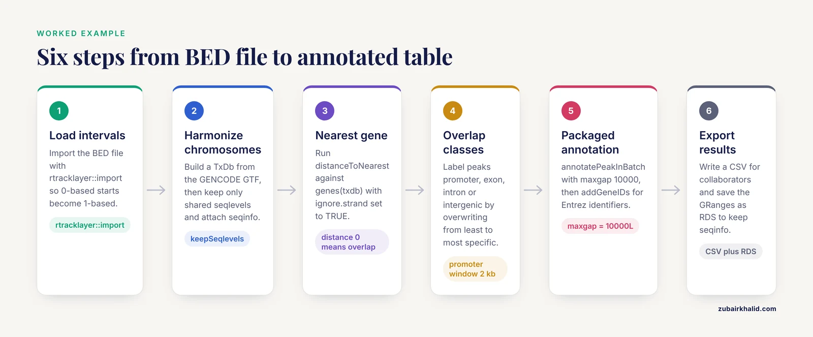
This walkthrough annotates a set of ChIP-seq or ATAC-seq peaks against human gene models. The same code annotates DMRs, QTL intervals, or any other ranges without modification.
Step 1: Load your intervals as a GRanges
The cleanest path from a BED file is rtracklayer::import, which converts BED 0-based coordinates to the 1-based convention R uses internally and preserves the extra BED columns:
library(rtracklayer)
peaks <- import("macs2_peaks.bed", format = "BED")
head(peaks, 3)
Expected output (values depend on your file):
GRanges object with 3 ranges and 2 metadata columns:
    seqnames            ranges strand |        name     score
       <Rle>         <IRanges>  <Rle> | <character> <numeric>
  [3]     chr1     994126-994626      * |   peak_1   142.5
  [4]     chr1   1038220-1038503      * |   peak_2    88.0
  [5]     chr1   1075235-1075735      * |   peak_3   201.3
  -------
  seqinfo: 25 sequences from an unspecified genome, no seqlengths
If your intervals are already in a data frame, use makeGRangesFromDataFrame() with keep.extra.columns = TRUE. If you built a GRanges by hand from a BED file by parsing columns yourself, remember that the BED chromStart column is 0-based, so add 1 to the start before constructing the IRanges. Forgetting this is one of the most common causes of off-by-one annotation errors, because every distance and overlap then shifts by a single base and boundary cases silently misclassify.
Check what came in before annotating:
length(peaks)                 # number of ranges
table(seqnames(peaks))        # distribution across chromosomes
summary(width(peaks))         # range widths, watch for width-1 surprises
Step 2: Attach a genome build and harmonize chromosome names
Overlaps and nearest-neighbor searches only work when both objects agree on chromosome names and lengths. Gene model sources disagree about whether chromosome 1 is written chr1 or 1, and they often include unplaced contigs that your peak file lacks. Resolve this with the seqinfo machinery:
library(GenomicFeatures)
txdb <- makeTxDbFromGFF("gencode.v44.annotation.gtf", format = "gtf")
makeTxDbFromGFF() parses the GTF into a TxDb object, a lightweight SQLite-backed transcript database that supports accessors such as genes(), transcripts(), exons(), cds(), and promoters(). This is the GenomicFeatures package doing its job as the transcript-structure layer of the range infrastructure [2]. During construction you may see a message that certain transcripts were excluded because their CDS locations could not be determined. That is normal for partially annotated transcripts, and the function reports how many were affected.
Now align the two objects:
library(GenomeInfoDb)
seqinfo(txdb)
seqlevels(peaks)

# keep only chromosomes present in both, in a consistent order
common <- intersect(seqlevels(peaks), seqlevels(txdb))
peaks  <- keepSeqlevels(peaks, common, pruning.mode = "coarse")
keepSeqlevels() with pruning.mode = "coarse" drops ranges on chromosomes you exclude, which is what you want when a peak file contains a scaffold the gene model does not. If your peak file uses chr1 and your GTF uses 1, rename before intersecting:
seqlevels(peaks) <- sub("^chr", "", seqlevels(peaks))Finally, attach the gene model's seqinfo to the peaks so that genome build metadata travels with the object:
seqinfo(peaks) <- seqinfo(txdb)If the two objects have genuinely incompatible sequence information, for example one says chr1 has length 248956422 and the other disagrees because you mixed hg38 with hg19, this assignment fails with an error telling you the sequence information is incompatible. That failure is protective. Fix the build mismatch rather than bypassing it.
Step 3: Annotate by nearest feature
The simplest annotation answers, for each peak, which gene is closest and how far away it is:
genes_gr <- genes(txdb)          # one range per gene, widest transcript span

hits <- distanceToNearest(peaks, genes_gr, ignore.strand = TRUE)
ann  <- as.data.frame(hits)
ann$gene_id <- genes_gr$gene_id[hits@subjectHits]

head(ann)
Expected output:
  queryHits subjectHits distance             gene_id
1         1        1204    38517 ENSG00000238009.6
2         2        1211        0 ENSG00000241833.4
3         3        1301     9274 ENSG00000225972.1
The distance column is the number of bases between the closest edges of the two ranges, with 0 meaning they touch or overlap. Rows where the peak lies inside a gene body report distance 0 against that gene. If a peak sits in a region with no gene model on the same chromosome within a huge span, distanceToNearest still returns the nearest hit on that chromosome, so distances can be very large. Distances are never reported across chromosomes.
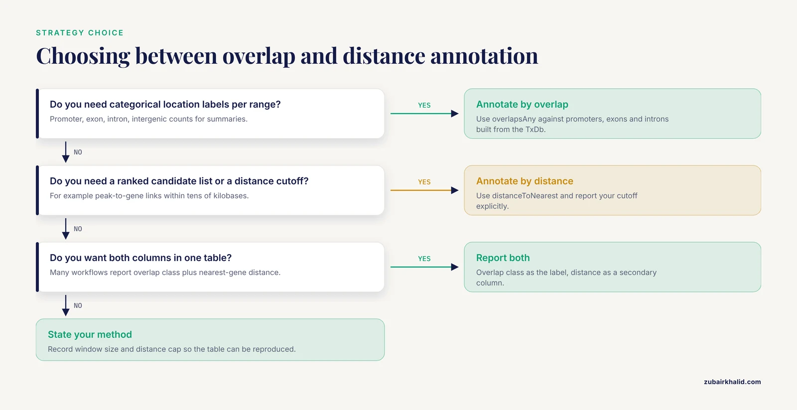
A practical threshold for peak-to-gene links in mammalian genomes is on the order of tens of kilobases, but the right cutoff depends on your assay and cell type. Report your cutoff explicitly, because a nearest-gene table built with a 10 kb cap and one built without a cap answer different questions.
Step 4: Annotate by overlap with feature classes
Nearest-gene annotation loses the distinction between a peak sitting in a promoter and one in the third intron. Overlap against labeled feature sets restores it. Build the feature sets from the same TxDb:
prom   <- promoters(txdb, upstream = 2000, downstream = 200)   # standard window
exons  <- exons(txdb, use.names = TRUE)
utr5   <- fiveUTRsByTranscript(txdb)                            # nested list
introns <- setdiff(transcripts(txdb), exons)                    # transcript minus exons
The promoter definition used above, 2 kb upstream through 200 bases downstream of the transcription start site, is a widely used convention in the peak annotation literature, and it is also the kind of default that dedicated annotation packages ship with [6]. State your window whenever you report promoter counts, because a 1 kb versus 5 kb definition changes the numbers materially.
Then classify each peak by priority, promoter first, then exon, then intron, then intergenic:
peaks$location <- "intergenic"
peaks$location[overlapsAny(peaks, introns, ignore.strand = TRUE)] <- "intron"
peaks$location[overlapsAny(peaks, exons,  ignore.strand = TRUE)] <- "exon"
peaks$location[overlapsAny(peaks, prom,   ignore.strand = TRUE)] <- "promoter"

table(peaks$location)
Expected output:
   exon intergenic   intron  promoter
    412       5298     3876       988
Note the assignment order. Overwriting from the least specific category to the most specific means a peak overlapping both a promoter and an exon is labeled promoter. If you want a one-to-many annotation instead, keep the Hits object from findOverlaps(peaks, prom) and work with the pairwise mapping rather than a single label per peak.
Step 5: Annotate with a dedicated package
The manual pipeline above teaches you the mechanics, but for production work there are purpose-built annotation packages. ChIPpeakAnno was developed specifically for batch annotation of enriched peaks from ChIP-seq, ChIP-chip, CAGE, or any experiment producing large numbers of enriched regions, with built-in summaries such as histograms of distances to nearest genes and significance testing of overlaps between replicate peak sets [6].
library(ChIPpeakAnno)
data(TSS.human.GRCh38)   # bundled transcription start site ranges

anno <- annotatePeakInBatch(peaks, AnnotationData = TSS.human.GRCh38,
                            output = "nearestLocation", maxgap = 10000L)
anno <- addGeneIDs(annotatedPeaks = anno, orgAnn = "org.Hs.eg.db",
                   IDs2Add = "entrez_id")
head(as.data.frame(anno))
output = "nearestLocation" returns the single nearest annotated feature per peak, and maxgap bounds the search so peaks far from any feature are reported as unannotated rather than joined to something tens of megabases away. Peaks with no feature inside maxgap carry an NA feature identifier, so filter or flag those rows deliberately.
FindIT2 extends the same annotation framework to multi-omics integration, supporting annotation of ChIP-seq and ATAC-seq peaks and identification of transcription factor targets by combining peak data with RNA-seq. Because it builds on the standard Bioconductor annotation classes, it can be applied to any species with genomic annotations, which makes it particularly useful for non-model organisms with less mature annotation resources [7].
Goldmine takes a complementary approach, annotating ranges from any source with gene model and feature context to support both global summaries and candidate-locus discovery, and has been used to characterize context patterns in transcription factor binding and differentially methylated regions [8].
Step 6: Export the annotated table
df <- as.data.frame(anno)
write.csv(df, "peaks_annotated.csv", row.names = FALSE)

# keep the GRanges too, for later range operations
saveRDS(anno, "peaks_annotated.rds")
The CSV goes to collaborators and spreadsheets. The RDS file preserves the full GRanges structure, including seqinfo and metadata columns, and is what you should feed into the next stage of your own pipeline.
Choosing an Annotation Strategy: A Summary Table
| Package | Key function | What it returns | Best used for |
|---|---|---|---|
| GenomicRanges | distanceToNearest() | One nearest hit per query with distance | Simple peak-to-nearest-gene tables |
| GenomicRanges | findOverlaps(), countOverlaps(), overlapsAny() | Pairwise hits, counts, or logical flags | Overlap classification against exons, promoters, TFBS, custom features |
| GenomicFeatures | genes(), promoters(), exons() | Feature GRanges from a TxDb | Building the reference feature sets |
| ChIPpeakAnno | annotatePeakInBatch() | Per-peak annotation against TSS or feature database | Batch annotation of large peak sets with distance summaries [6] |
| ChIPpeakAnno | addGeneIDs() | Peaks joined to symbol, Entrez, Ensembl IDs | Preparing tables for enrichment tools |
| FindIT2 | peak and TF-target functions | Annotated peaks, TF-target links | Integrating peak annotation with RNA-seq for TF target inference [7] |
| Goldmine | context annotation functions | Ranges with gene and feature context | Quick global context for arbitrary range sets [8] |
| GenomicInteractions | annotateInteractions() | Interactions labeled by node annotation | Hi-C and ChIA-PET interaction data [1] |
| RaggedExperiment | qreduceAssay() | Rectangular assay matrix over fixed ranges | Per-sample ragged data such as mutations and CNV converted to matrices [4] |
| nullranges | bootRanges(), matchRanges() | Null range sets | Enrichment testing with matched or bootstrapped controls [4][6] |
Checking That Your Annotation Is Correct
Validation is cheap and catches most errors. Run these checks every time.
First, confirm the coordinates agree by testing a known case. Take a well-annotated gene, for example MALAT1 on human chromosome 11, create a range covering its start position from your gene model, and verify that distanceToNearest returns distance 0 to that same gene. A mismatch means coordinate conventions or builds disagree.
Second, verify the coordinate system round trip. Export a few ranges with export(peaks[1:5], "check.bed"), view them in a genome browser, and confirm they land where the original peak caller placed them. This single check catches both the 0-based versus 1-based error and whole-chromosome naming errors.
Third, sanity-check the distributions. In a typical mammalian ChIP-seq experiment for a transcription factor, a large fraction of peaks should land in promoter-proximal windows, but enhancer-biased factors will show much lower promoter fractions. The point is not to enforce a target number, it is that an annotation in which nearly every peak is intergenic usually signals a build or naming mismatch, while one in which nearly every peak is promoter-proximal can signal that your promoter window swallowed the genome.
Fourth, count the NAs. After annotatePeakInBatch or a capped distanceToNearest, explicitly count unannotated ranges:
sum(is.na(anno$feature))If that number is unexpectedly high, revisit maxgap, chromosome harmonization, and the gene model completeness for your build.
Fifth, confirm the gene identifier mapping did not silently fail. addGeneIDs() warns when identifiers do not match, but scanning head() output for a column full of NAs is faster. Identifier mapping depends on matching versions of the TxDb and the organism database, so regenerate both from the same Bioconductor release when possible.
Beyond Peaks: Annotating Other Range Types
The peak-centric workflow is the most common case, but the same infrastructure annotates more complex objects.
Genomic interactions
Hi-C, ChIA-PET, and related assays produce pairs of interacting loci rather than single ranges. The InteractionSet package provides Bioconductor classes that represent genomic interactions and their associated experimental data, built on the standard range infrastructure so that higher-level packages can share one representation [9]. The GenomicInteractions package builds on this to allow annotation and summarization of large genome-wide interaction datasets at the level of individual interactions and feature sets, demonstrated on Hi-C and ChIA-PET data [3]. In practice you build a GInteractions object with two anchor GRanges, call annotateInteractions() against feature databases such as promoters and enhancers, and then summarize promoter-to-enhancer counts with a single call. The r3Cseq package similarly supports the discovery and annotation of long-range interactions from 3C-seq data, from aligned reads through normalization to visualization of candidate interaction regions [5].
Per-sample ragged ranges
Variant calls, copy number segments, methylation blocks, and open chromatin regions differ in coordinates from sample to sample. This ragged structure resists the rectangular matrices that downstream statistics expect. RaggedExperiment solves this by providing a lossless representation of disparate genomic ranges across specimens alongside efficient reshaping into rectangular summaries, with demonstrated applications to somatic mutation, copy number, methylation, and open chromatin data across 33 TCGA cancer datasets [4]. Annotating such data then becomes a two-stage process, first annotate the union range space against gene models, then use qreduceAssay() to project each sample onto that shared space.
Null ranges for enrichment testing
Once you have annotated a peak set, the obvious follow-up question is whether the annotation, for example the number of peaks in enhancers, is more than expected by chance. Naive random shuffling treats the genome as uniformly distributed with respect to gene density, chromatin state, and mappability, which it is not. Two Bioconductor resources address this directly. matchRanges generates null hypothesis ranges via propensity score-based covariate matching from a background pool, controlling for multiple covariates at once within the standard range data classes [10]. bootRanges generates bootstrapped null sets for enrichment analysis and shows that shuffling or permutation schemes can produce overly narrow null distributions, while a block bootstrap that preserves local genomic correlation structure yields more reliable nulls [11]. If you report an enrichment fold change, report it against one of these matched or bootstrapped nulls rather than against uniform shuffling.
Common Mistakes and Limitations
These are the errors that invalidate interval annotation most often, in rough order of frequency.
Mixing genome builds. Annotating hg19 peaks against an hg38 gene model produces plausible-looking output with wrong answers, because homologous coordinates still overlap some genes. There is no warning by default unless seqinfo lengths conflict. Prevent it by carrying seqinfo end to end and by checking genome(peaks) against genome(txdb) explicitly.
Chromosome naming style mismatches. chr1 versus 1, and the extra chr1_KI270706v1_random style contigs in UCSC references, cause peaks to vanish silently from overlap queries because nothing matches on those chromosomes. Always compare table(seqnames(peaks)) before and after annotation and account for every chromosome. The GenomeInfoDb functions seqlevelsStyle() and keepSeqlevels() are the intended fixes.
BED coordinate confusion. BED chromStart is 0-based. GRanges start is 1-based. rtracklayer::import() converts correctly, manual parsing does not. If you must parse manually, add 1 to BED starts and document that you did.
Strand handling. Peak callers typically report strand *, and gene models report + or -. findOverlaps() defaults to strand-aware matching, so an unstranded peak set can fail to overlap anything if you do not pass ignore.strand = TRUE. Conversely, when annotating stranded libraries such as nascent transcription data, strand awareness is what you want, and ignore.strand = TRUE would be the bug.
Misreading maxgap and minoverlap. In findOverlaps(), minoverlap is the minimum number of overlapping bases required, not a distance. In distanceToNearest() there is no cap unless you filter afterward. Read the argument definitions for the function you are calling, because the same parameter name means different things across functions.
Equating the nearest gene with the regulatory target. Nearest-gene assignment is a first-pass annotation, not a causal target assignment. A peak 40 kb from the nearest gene can regulate a gene 200 kb away, and a peak inside a gene body can regulate a neighboring gene. Use nearest-gene tables for descriptive context and confirm putative targets with co-accessibility, interaction data, or perturbation experiments. Tools such as FindIT2 exist precisely because target inference requires more than proximity [7].
Losing metadata through range operations. reduce(), disjoin(), and similar operations can merge or split ranges, and the metadata columns of the inputs do not transfer to merged outputs in an obvious way. Annotate after range arithmetic, or track provenance explicitly.
Ignoring unplaced and alternate contigs. Peaks on chrUn, _alt, and _random contigs inflate intergenic fractions when the gene model lacks those contigs, or double-count when it includes them. Decide your policy, usually to exclude them, state it, and apply it before annotation.
Version churn. Gene models change between GENCODE releases. Peaks near genes whose annotation was revised will shift annotation labels between releases. Record the gene model release, the TxDb or EnsDb version, the Bioconductor release from BiocManager::version(), and the genome build in every script and report. None of this tooling substitutes for biological judgment, and any annotation used for a decision that matters should be reviewed by someone with domain knowledge of the locus or biology involved.
Tips for Faster, More Reproducible Annotation
- Pin one Bioconductor version per project. Run
BiocManager::version()at the top of the script and print it into the output log. Mixed versions are a leading cause of annotation tables that cannot be regenerated. - Cache downloaded annotations.
AnnotationHub()caches resources locally after the first download, so a repeat run is offline-safe and fast. For fully reproducible containers, pre-populate the cache during image build. - Prefer set operations over loops.
overlapsAny(),countOverlaps(), andsubsetByOverlaps()vectorize across thousands of ranges. A per-peakforloop callingfindOverlaps()one range at a time is slower by orders of magnitude. - Keep the
Hitsobjects.findOverlaps()results are lightweight and let you recompute counts, first hits, and joined tables without repeating the search. - Save intermediate
GRangesas RDS. Text exports lose seqinfo and strand-type information. Save both an RDS for the pipeline and a CSV for humans. - For non-model organisms, build the TxDb from your own GFF3 or GTF with
makeTxDbFromGFF(). The Bioconductor range infrastructure is organism-agnostic, and FindIT2 explicitly leverages this to support species with any available genomic annotation [7].
Frequently Asked Questions
What does it mean to annotate genomic ranges in R?
It means taking a set of genomic intervals held as a GRanges object and attaching biological context to each one, such as the nearest gene, the distance to that gene, whether the interval overlaps a promoter, exon, or other annotated feature, and standardized gene identifiers. The Bioconductor range infrastructure provides the data structures and overlap algorithms that make this efficient [2].
Which Bioconductor package should I start with?
Start with GenomicRanges, since it defines the GRanges container and the overlap and nearest-neighbor functions everything else uses [2]. Add GenomicFeatures for building gene model feature sets, rtracklayer for reading BED and GTF files, and ChIPpeakAnno once you want packaged peak annotation with summaries and identifier mapping [6].
How do I convert a BED file to a GRanges object?
Use rtracklayer::import("file.bed", format = "BED"). This converts BED 0-based half-open coordinates to the 1-based convention used inside R and preserves the name and score columns as metadata. Avoid parsing BED columns manually into GRanges unless you adjust the start coordinate by one base.
How do I find the nearest gene to each range?
Build a gene GRanges from a TxDb with genes(txdb), then call distanceToNearest(peaks, genes_gr, ignore.strand = TRUE). The returned object maps each query range to its nearest gene index with the gap distance in bases, zero when the range lies inside the gene span [2].
Should I annotate by overlap or by distance?
Use overlap when you want categorical location labels such as promoter, exon, or intron, and distance when you want a ranked candidate list or need to impose an explicit genomic distance cutoff. Many workflows report both, overlap class for each peak and nearest-gene distance as a secondary column [6].
Where do I get reliable gene annotations?
From versioned, curated sources. Options include a GENCODE or Ensembl GTF converted with makeTxDbFromGFF(), prebuilt TxDb packages on Bioconductor, and Ensembl-derived EnsDb objects retrieved through AnnotationHub. Whichever you choose, record the exact release version, because annotation labels shift between gene model releases [7].
How do I handle chromosome name mismatches like chr1 versus 1?
Harmonize the seqlevels of both objects before any overlap or distance call, using sub() on the level names or seqlevelsStyle(), then restrict both objects to the chromosomes they share with keepSeqlevels() and attach a common seqinfo. Unmatched chromosomes cause silent misses, so verify with table(seqnames()) before and after.
Can I annotate ranges in species without a prebuilt Bioconductor annotation database?
Yes. If your species has a genome assembly and a GFF3 or GTF gene model, makeTxDbFromGFF() builds a TxDb locally and the entire GenomicRanges annotation workflow applies unchanged. Packages such as FindIT2 are designed to work with any species that has genomic annotations, which makes this route practical for non-model organisms [7].
Sources
- Orchestrating high-throughput genomic analysis with Bioconductor
- Software for Computing and Annotating Genomic Ranges
- GenomicInteractions: An R/Bioconductor package for manipulating and investigating chromatin interaction data.
- RaggedExperiment: the missing link between genomic ranges and matrices in Bioconductor
- r3Cseq: an R/Bioconductor package for the discovery of long-range genomic interactions from chromosome conformation capture and next-generation sequencing data
- ChIPpeakAnno: a Bioconductor package to annotate ChIP-seq and ChIP-chip data
- FindIT2: an R/Bioconductor package to identify influential transcription factor and targets based on multi-omics data
- Goldmine integrates information placing genomic ranges into meaningful biological contexts
- Infrastructure for genomic interactions: Bioconductor classes for Hi-C, ChIA-PET and related experiments.
- matchRanges: generating null hypothesis genomic ranges via covariate-matched sampling
- bootRanges: flexible generation of null sets of genomic ranges for hypothesis testing