AlphaFold Output Files Explained
By Dr. Zubair Khalid, DVM, MS, PhD ·

By the end of this article you will be able to name every file an AlphaFold2, ColabFold, AlphaFold3, or AlphaFold Server run produces, know which file to open first, extract pLDDT, PAE, pTM, and ipTM from the right place, rank your models on defensible grounds, convert outputs between PDB and mmCIF, and run a quick sanity check on your results. You will need Python 3.9 or newer with NumPy and Matplotlib, any text editor, and either a completed prediction from the AlphaFold2 repository or ColabFold on your own machine or a browser account on the AlphaFold Server. If you have never run a prediction yet, you can still follow along because every file below is small enough to inspect with plain text tools.
The models themselves get most of the attention, but the sidecar files carry the information that decides whether you should trust the model. A ranked PDB file without its confidence JSON is a set of coordinates with no error model attached. A beautiful PAE plot is worthless if you misread which chain is which. This guide covers all of it in one place.
What a Prediction Produces at a Glance
Every AlphaFold flavor writes coordinates plus one or more confidence sidecars. The table below maps the main file families to where you find them and how you read them.
| File type | Produced by | Contents | Read it with |
|---|---|---|---|
| ranked PDB files | AlphaFold2 repo, ColabFold | Ranked models, pLDDT in the B-factor column | PyMOL, ChimeraX, any PDB parser |
| unrelaxed and relaxed PDB files | AlphaFold2 repo, ColabFold | Coordinates before and after Amber energy minimization | Same as above |
| result NPZ | AlphaFold2 repo | pLDDT array, PAE matrix, distogram as compressed NumPy arrays | Python with NumPy |
| scores JSON | ColabFold, AlphaFold2 repo (recent versions) | pTM, ipTM, per-residue pLDDT, full PAE matrix | Python with json |
| mmCIF model files | AlphaFold3, AlphaFold Server | Coordinates with per-atom confidence, ligands, nucleic acids, ions | PyMOL, ChimeraX, gemmi |
| summary confidence JSON | AlphaFold3, AlphaFold Server | Per-chain pTM, per-chain ipTM, chain-pair ipTM matrix | Python with json, any text editor |
| full data JSON | AlphaFold3, AlphaFold Server | PAE and predicted distance error matrices over all tokens | Python with json |
| MSA and feature files | AlphaFold2 repo, ColabFold | Alignment in A3M or Stockholm format, database provenance, pickled features | Text editor, pickle viewer |
The rest of the article walks through each family in the order you will actually use them.
AlphaFold2 Output Files Explained Step by Step
This section uses ColabFold for the walkthrough because it is the easiest way to run AlphaFold2 locally and it writes the same core file types as the original repository. The exact filenames vary slightly between versions, so treat the patterns below as a template rather than a contract.
Step 1: Run a prediction and keep every file it writes
colabfold_batch myprotein.fasta results/colabfold_batch is the command line driver for ColabFold. In one pass it searches the sequence databases for homologs, builds a multiple sequence alignment, runs the five AlphaFold2 models, ranks the results, and writes everything into the directory you name. For a two-chain complex you supply a FASTA file with two entries separated by a chain break marker, and ColabFold switches to the multimer models automatically.
A completed run leaves a directory that looks roughly like this:
$ ls -lh results/
total 2.4M
-rw-r--r-- 1 you you  21K Jan 14 10:02 myprotein.a3m
-rw-r---- 1 you you  412 Jan 14 10:02 myprotein.env
-rw-r--r-- 1 you you  87K Jan 14 10:06 myprotein_unrelaxed_rank_001_alphafold2_multimer_v3_model_1_seed_000.pdb
-rw-r--r-- 1 you you  87K Jan 14 10:06 myprotein_unrelaxed_rank_002_alphafold2_multimer_v3_model_2_seed_000.pdb
-rw-r--r-- 1 you you  87K Jan 14 10:06 myprotein_unrelaxed_rank_003_alphafold2_multimer_v3_model_3_seed_000.pdb
-rw-r--r-- 1 you you  87K Jan 14 10:06 myprotein_unrelaxed_rank_004_alphafold2_multimer_v3_model_4_seed_000.pdb
-rw-r--r-- 1 you you  87K Jan 14 10:06 myprotein_unrelaxed_rank_005_alphafold2_multimer_v3_model_5_seed_000.pdb
-rw-r--r-- 1 you you 310K Jan 14 10:06 myprotein_scores_rank_001_alphafold2_multimer_v3_model_1_seed_000.json
-rw-r--r-- 1 you you 310K Jan 14 10:06 myprotein_scores_rank_002_alphafold2_multimer_v3_model_2_seed_000.json
If you enable relaxation with the appropriate ColabFold flag, you additionally get one relaxed PDB per rank. The .env file records which databases, versions, and timestamps produced the alignment. The .a3m file holds the multiple sequence alignment. Do not delete these even after you have your model. They are your provenance record and they tell you how deep the alignment was, which is one of the strongest predictors of prediction quality.
Step 2: Decode the ranked PDB files and the B-factor column
The five unrelaxed PDB files are the five model predictions sorted best first. ColabFold and the AlphaFold2 repository rank monomer predictions by mean pLDDT and multimer predictions by a composite score described below. The filename tells you the rank, the model number, and the random seed.
Open any of these files in a text editor and look at the ATOM records. The last numeric column before the element symbol is the B-factor column, and AlphaFold repurposes it to store pLDDT:
ATOM    563  CA  ALA A  71      12.304  -8.612   3.902  1.00 94.12           C
ATOM    571  CA  GLY A  72      11.447  -7.908   6.871  1.00 91.85           C
ATOM    579  CA  LYS A  73       9.912  -5.103   8.551  1.00 63.27           C
pLDDT stands for predicted local distance difference test. It is a per-residue score from 1 to 100 that estimates how well each residue position matches the true structure on a local scale, roughly within the neighborhood of that residue. The standard reading, taken from the AlphaFold Database help documentation, is that residues above 90 are modeled with very high accuracy, residues from 70 to 90 have an accurately predicted backbone, residues from 50 to 70 are low confidence and often flexible or disordered, and residues below 50 should be treated as unreliable and frequently correspond to intrinsically disordered regions.
Notice that the third residue in the snippet above drops from 91.85 to 63.27. That is the confidence dropping over a loop. When you load the file in PyMOL, the default representation colors the model by these B-factors, which is why AlphaFold models appear blue in well-predicted cores and orange or red in loops. That coloring is not decoration. It is the error model rendered on the structure.
Step 3: Open the scores JSON
Each rank has a JSON sidecar. This is the file to open first when you want a verdict, because it contains the global and per-residue confidence numbers in plain text.
import json

with open("results/myprotein_scores_rank_001_alphafold2_multimer_v3_model_1_seed_000.json") as f:
    s = json.load(f)

print("pTM:", round(s["ptm"], 3))
print("ipTM:", round(s["iptm"], 3))
print("max pTM:", round(s["max_ptm"], 3))
print("max ipTM:", round(s["max_iptm"], 3))
print("pLDDT array length:", len(s["plddt"]))
Expected output for a well-behaved homodimer:
pTM: 0.861
ipTM: 0.784
max pTM: 0.869
max ipTM: 0.792
pLDDT array length: 342
The keys to know:
ptm, the predicted TM-score. A scalar from 0 to 1 estimating the global structural similarity between the predicted model and the unknown true structure. Global here means the whole assembly is compared at once.iptm, the interface predicted TM-score. Present when you predict multiple chains. It scores only the interchain part of the model and is the primary number to check for protein-protein interaction predictions.max_ptmandmax_iptm, variants that score only the best-aligning receptor-ligand pair within a multimer. They matter for antibody-antigen and other asymmetric complexes.plddt, the per-residue confidence array, matching the B-factor column of the corresponding PDB one residue at a time.pae, the full predicted aligned error matrix, described next.
Step 4: Read the predicted aligned error matrix
The predicted aligned error, PAE, is a matrix with one row and one column per residue or per token. Entry (i, j) estimates, in angstroms, the expected position error at residue j if you align the prediction to the true structure using residue i as the anchor. Low values between two residues mean the model is confident about their relative position. High values mean the model does not know where they sit relative to each other, even if both residues individually have high pLDDT.
For a two-chain prediction, the PAE matrix has a visible block structure. The two diagonal blocks are intra-chain errors. The two off-diagonal blocks are interchain errors, and those are the blocks that tell you whether the predicted interface is real or a guess.
import json
import numpy as np

with open("results/myprotein_scores_rank_001_alphafold2_multimer_v3_model_1_seed_000.json") as f:
    s = json.load(f)

pae = np.array(s["pae"])
print("PAE matrix shape:", pae.shape)

chain_a_len = 171
chain_b_len = 171

inter_AB = pae[:chain_a_len, chain_a_len:]
inter_BA = pae[chain_a_len:, :chain_a_len]

print("Mean A-to-B interface PAE:", round(inter_AB.mean(), 2), "angstroms")
print("Fraction of interface pairs below 5 A:",
      round((inter_AB < 5).mean() * 100, 1), "percent")
Expected output:
PAE matrix shape: (342, 342)
Mean A-to-B interface PAE: 3.41 angstroms
Fraction of interface pairs below 5 A: 88.4 percent
In ColabFold plots, the PAE values are shown on a color scale that runs up to roughly 32 angstroms, which matches the cap that AlphaFold2 applies to the metric. A dark off-diagonal block, meaning low interchain PAE, is the strongest visual evidence that two chains were placed with a defined relative orientation. A pale, washed-out off-diagonal block with good per-chain diagonal blocks means each chain folded nicely in isolation but the model has no real basis for the interface you are looking at.
To plot the matrix yourself:
import matplotlib.pyplot as plt

plt.imshow(pae, cmap="viridis", vmin=0, vmax=30)
plt.colorbar(label="Expected position error (angstroms)")
plt.xlabel("Scored residue")
plt.ylabel("Aligned residue")
plt.savefig("pae_rank_001.png", dpi=300)
Step 5: Understand the MSA files
The .a3m file is a text-format multiple sequence alignment. The first line is a header, the second line is the query sequence, and each following pair of lines is one homologous sequence. Lowercase letters inside a sequence mark insertions relative to the query, which is how the A3M format compresses gapped alignments. You can count effective sequences with a one-liner and use alignment depth as a quick quality flag, because predictions built on shallow alignments tend to come with worse PAE and more scattered model rankings.
grep -c "^>" results/myprotein.a3mThe .env file is a single record listing the databases searched and the dates of those searches. Keep it. When a reviewer or collaborator asks how the prediction was made six months later, this file answers the question.
Step 6: Relaxed versus unrelaxed models
By default, AlphaFold2 emits unrelaxed models, meaning coordinates straight from the network with no energy minimization. These can contain small steric clashes and slightly strained bond geometry. Relaxation runs the model through the Amber force field to clean up local geometry. ColabFold adds relaxation when you request it, and the original repository offers Amber relaxation or a lighter GPU-based relaxation option. The relaxed model is the one you want for downstream molecular mechanics work such as binding energy calculations, because those methods are sensitive to clashes. For visualization and most analysis, the difference is small but real. Always record in your notes whether a figure or a number came from the relaxed or unrelaxed file, because the two are not interchangeable in detail.
The Original AlphaFold2 Repository Output
If you run the deepmind/alphafold codebase directly instead of ColabFold, the command looks like this:
python run_alphafold.py \
  --fasta_paths=myprotein.fasta \
  --output_dir=results \
  --model_preset=multimer \
  --db_preset=full_dbs \
  --num_multimer_predictions_per_model=5 \
  --use_gpu_relax=true
The output directory then contains:
unrelaxed_model_1_multimer.pdbthroughunrelaxed_model_5_multimer.pdb, one per model, before rankingrelaxed_model_1_multimer.pdband so on, if relaxation was enabledranked_0.pdbthroughranked_4.pdb, the ranked copies, withranked_0.pdbbeing the top modelresult_model_1_multimer.npz, a compressed NumPy archive holding pLDDT, the PAE matrix, and the distogram for each modeltimings_model_1_multimer.json, a small file recording how long each stage took- a
msasdirectory with the alignment files and a pickled features object that records every input the network saw
The NPZ file is the raw confidence store for this pipeline:
import numpy as np

d = np.load("results/result_model_1_multimer.npz")
print(sorted(d.keys()))
print("pLDDT shape:", d["plddt"].shape)
print("PAE shape:", d["pae"].shape)
Expected output for the same 342-residue dimer:
['atom_plddts', 'distogram', 'mask', 'pae', 'plddt', 'structure_module']
pLDDT shape: (342,)
PAE shape: (342, 342)
The distogram entry holds the model's predicted distance distribution between residue pairs. Most users never touch it, but it is the underlying object from which interface contact maps can be reconstructed if you want to go deeper than PAE.
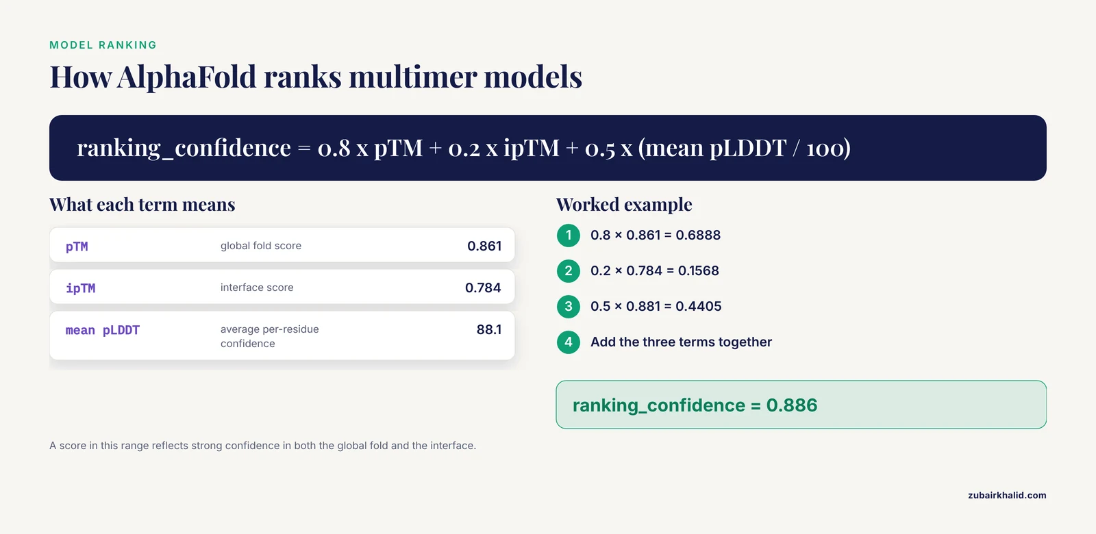
Ranking works as follows. For monomers, models are sorted by mean pLDDT. For multimers, the AlphaFold-Multimer pipeline ranks by a composite confidence called ranking_confidence:
ranking_confidence = 0.8 x pTM + 0.2 x ipTM + 0.5 x (mean pLDDT divided by 100)
Worked example for the dimer above: 0.8 x 0.861 + 0.2 x 0.784 + 0.5 x 0.88 = 0.6888 + 0.1568 + 0.44 = 0.886. A composite score in this range reflects strong confidence in both the global fold and the interface.
AlphaFold3 Output Files
AlphaFold3 changed two things that matter for output files. First, it writes mmCIF rather than PDB, which is necessary because AF3 models nucleic acids, ligands, metal ions, and covalent modifications alongside proteins, and the older PDB format cannot represent those cleanly. Second, it restructures the confidence reporting around per-chain and per-chain-pair metrics.
A completed AF3 run, whether local or through the server, gives you:
- One model CIF file per sampled prediction, with per-atom confidence values stored in the B-factor-like field
- A summary confidences JSON containing
chain_ptmfor every chain,chain_iptmfor every chain, andchain_pair_iptm, a matrix giving the interface score for every ordered pair of chains - A full data JSON containing the token-level PAE matrix and the predicted distance error, PDE, which estimates the error in the distance between a pair of atoms
- Supporting files with the MSA and template data used for the run
The per-chain-pair ipTM matrix is a genuine improvement for large assemblies. In a five-chain complex, a single global ipTM number can hide the fact that chains three and five form a confident subcomplex while chain two floats unanchored. Reading chain_pair_iptm row by row shows you immediately which interfaces are supported and which are speculative.
The ipTM definition itself carries over from AlphaFold2, and that matters. Because AF3 computes ipTM over whole chains, the same construct-design sensitivity described for AF2 applies to AF3 results as well, which the next section explains with numbers.
AlphaFold Server: What You Download and How to Read It
The AlphaFold Server at alphafoldserver.com is the hosted interface to AlphaFold3, offered by Google DeepMind and the Institute for Protein Design collaboration for non-commercial use. You build a job in the browser by pasting sequences and declaring each entity type as protein, DNA, RNA, ligand, or ion. The server runs the prediction and hands you a downloadable archive.
Inside the archive you get the mmCIF model files, the summary and full confidence JSON files described above, and the input artifacts such as alignment data. The workflow differences from a local run are worth noting. The server enforces job quotas per user, it accepts a bounded total length across all entities in a single job, and you cannot install custom databases or change sampling parameters the way you can locally. In exchange, you get ligand and nucleic acid modeling with zero setup.
A practical server workflow: submit the same complex two or three times rather than once, because each submission samples models, and consistency across submissions is your cheapest check on whether a predicted interface is stable. If the same contact appears with low interchain PAE in three independent jobs, the interface has support. If each job invents a different orientation, treat all of them as hypotheses.
Confidence Metrics Reference
| Metric | Range | Stored in | What it measures | Rough reading |
|---|---|---|---|---|
| pLDDT | 1 to 100 | PDB B-factor column, JSON plddt key | Local accuracy around each residue | Above 90 very high, 70 to 90 confident backbone, below 70 increasingly unreliable |
| PAE | 0 to about 32 angstroms | JSON pae, NPZ pae | Relative position error between residue pairs given an alignment on one of them | Interchain blocks below 5 angstroms indicate a defined interface |
| pTM | 0 to 1 | scores JSON | Global fold accuracy of the whole assembly | Values above 0.8 generally indicate a well-modeled assembly |
| ipTM | 0 to 1 | scores JSON | Accuracy of interchain geometry only | The headline number for interaction predictions, with the caveat below |
| ranking_confidence | 0 to 1 | implied by file ranking order | Composite used to sort multimer models | The number behind the rank in the filename |
One caution on thresholds. The AlphaFold-Multimer paper suggested treating ipTM values near or above roughly 0.8 as high-confidence interfaces and values below about 0.6 as low confidence, and many groups use these cutoffs as a first screen. Treat them as screening heuristics rather than probabilities, for the reason documented in the next section.
The ipTM Problem You Need to Know About
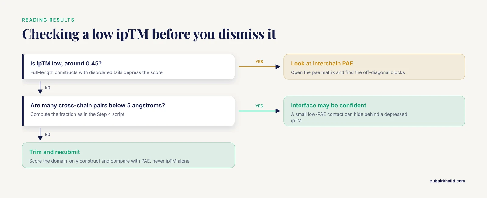
The ipTM score is the number most people quote when they claim that AlphaFold predicts an interaction. It has a well-documented weakness that directly affects how you should read your output files. In the mathematical formulation used by both AlphaFold2 and AlphaFold3, ipTM scores the interaction of whole chains. If either chain in a predicted complex carries long disordered regions or accessory domains that are not part of the interface being studied, those residues drag the ipTM score down even when the interface itself is predicted perfectly well. The score then fails at its two jobs at once. It understates the accuracy of the predicted interface geometry, and it can mislead you about whether two proteins actually interact.
The practical symptom is easy to recognize. You predict a full-length construct pair from UniProt sequences and get an ipTM of 0.45. You trim both sequences down to the interacting domains, resubmit the identical core, and the ipTM jumps to 0.75, even though the model of the interface itself has not changed. A 2025 analysis by Dunbrack demonstrated this behavior and showed it follows directly from how ipTM averages over all residue pairs across the full chains [1].
The same work proposed a concrete fix that changes how the score should be computed [1]:
- Include in the ipTM calculation only residue pairs whose interchain PAE values are good.
- Adjust the d0 parameter in the TM-score equation, which normally scales with full sequence length, so it reflects only the count of residues with well-predicted interchain relationships.
- Use the PAE values themselves rather than the full probability distributions over aligned error when computing the pairwise residue-residue pTM contributions.
For you as a user of existing output files, the operating lesson is this: when ipTM looks low, check the interchain PAE block before you believe or dismiss the number. Compute the fraction of cross-chain residue pairs with PAE under 5 angstroms, as in the Step 4 script. A construct where a small fraction of residue pairs have very low PAE, concentrated in the domain-domain contact, can be a confident prediction hiding behind a depressed ipTM. Conversely, an ipTM of 0.7 built on full-length chains with disordered tails is not comparable to an ipTM of 0.7 on a trimmed construct, so never compare the two directly.
Common Mistakes and Limitations
Judging a complex by pLDDT alone. pLDDT is a per-residue local score. Two chains can each average 92 pLDDT while sitting next to each other in a random orientation. The interface verdict lives in the interchain PAE blocks and ipTM, never in pLDDT. Read all three numbers together.
Trusting ipTM on full-length chains without looking at PAE. As documented above, disordered regions and non-interacting accessory domains inside the submitted constructs depress ipTM and can invert the interpretation of a prediction [1]. When your construct includes long low-pLDDT tails, the ipTM in the output file is answering a question you did not ask.
Comparing ipTM across differently trimmed constructs. Because the score formulation depends on chain composition and length through the d0 parameter, an ipTM from a domain-only construct is not on the same scale as one from the full-length protein [1]. If you want a defensible comparison, score every construct with the same trimming scheme or use a PAE-filtered reimplementation of the metric.
Losing the B-factor column through editing. Many PDB manipulation tools rewrite or zero the B-factor column during renumbering, chain renaming, or format conversion. The moment that column is stripped, the per-residue confidence is gone from the file. Convert with tools that preserve it, or reattach the pLDDT array from the JSON before the file leaves your pipeline.
Reading ranked_0 as truth and ignoring the other four models. AlphaFold samples. Rank two can disagree with rank one about an interface orientation, and disagreement between top models is information. A common and defensible practice is to run several seeds, compare the top-ranked interfaces across seeds, and report the consensus or the spread.
Interpreting low PAE between two residues as proof of a specific contact. PAE says the model is confident about the relative geometry of two positions. Confident placement of a wrong hypothesis is possible, particularly with shallow MSAs. Cross-check interfaces against known biology, mutagenesis data, or experimental structures where they exist.
Mixing relaxed and unrelaxed models in downstream analysis. If you compute interface areas or run binding energy estimates, use one relaxation state consistently. Relaxed and unrelaxed coordinates differ enough at contact distances to change the numbers.
Forgetting that AlphaFold predicts one state. These models output a single conformation per prediction. Proteins known to switch between conformational states, allosteric switches, and conditionally folded regions will show low pLDDT in the regions that change state, which is a limitation of the method rather than an error in your files. The low-confidence region may be real biology telling you the region is flexible.
Practical Tips
Summarize a whole run in one pass. Before opening any structure, collect the headline numbers for every rank in a table:
import glob
import json

rows = []
for path in sorted(glob.glob("results/*_scores_rank_*.json")):
    with open(path) as f:
        s = json.load(f)
    rows.append((
        path.split("rank_")[1][:3],
        round(s["ptm"], 3),
        round(s["iptm"], 3),
        round(sum(s["plddt"]) / len(s["plddt"]), 1),
    ))

for r in sorted(rows):
    print(r, "pTM", r[1], "ipTM", r, "mean pLDDT", r)
Expected output:
001 pTM 0.861 ipTM 0.784 mean pLDDT 88.1
002 pTM 0.855 ipTM 0.771 mean pLDDT 87.6
003 pTM 0.849 ipTM 0.753 mean pLDDT 87.0
004 pTM 0.842 ipTM 0.699 mean pLDDT 86.4
005 pTM 0.831 ipTM 0.682 mean pLDDT 85.9
Compute interface pLDDT for the residues that matter. The mean pLDDT over the whole complex rewards a beautiful domain next to a meaningless contact. Restrict the average to residues within 6 angstroms of the partner chain, computed with any standard structural neighbor tool, and you get a number that tracks interface quality rather than global fold quality.
Keep the seed and version with the file. ColabFold embeds model version and seed in the filename, which is exactly why the filenames are long. When you rename files for a project, carry that information into the new name or a sidecar text file. A coordinate file whose sampling conditions are unknown is close to worthless for publication.
Validate before you trust. pLDDT measures agreement between the model and its own uncertainty, not physical correctness. Run a geometry check such as MolProbity through Phenix or a similar validation tool on your top model, especially if the structure will be used for docking or design. After Amber relaxation, clashes should drop substantially, and a validation report will confirm it.
Convert formats without losing confidence data. If your downstream tool requires PDB and your model is mmCIF from AF3, convert with gemmi, which preserves the confidence field:
gemmi convert model_0.cif model_0.pdbThen verify that the B-factor column of the converted file still shows the characteristic spread from around 30 to the high 90s rather than a flat line of zeros.
For ligands and nucleic acids, prefer AF3-class outputs. AF2 writes protein-only PDB files. If your system includes an ATP molecule, a zinc ion, or an RNA strand, the AF3 output files are the correct starting point, and the per-chain-pair ipTM matrix is the file to check for whether the ligand or nucleic acid placement is supported.
Frequently Asked Questions
Where is pLDDT stored in an AlphaFold output file?
In the B-factor column of the PDB or mmCIF file, one value per residue or per atom. Open the file in a text editor and read the last numeric column of each ATOM record, or load the structure in PyMOL where the default color scheme maps that column to blue, cyan, yellow, and orange by confidence tier.
What is the difference between ranked_0.pdb and relaxed_0.pdb?
The ranked file is the top-scoring model as produced by the network before any energy minimization, and the relaxed file is that same model after Amber force field relaxation to remove clashes and clean up geometry. Coordinates differ slightly, so pick one state and use it consistently across all analyses in a project.
What is a good ipTM score?
As a rough screen, values around or above 0.8 suggest a confident interface and values below roughly 0.6 suggest a weakly supported one, but the cutoffs are heuristics rather than probabilities. Because ipTM is computed over whole chains, disordered tails and extra domains depress the score, so always cross-check the interchain PAE block before accepting or rejecting an interface [1].
Why did my ipTM go up when I removed domains from my construct?
Because ipTM averages over all residue pairs across the full chains, and removing residues that are not part of the interface removes low-quality terms from that average. The Dunbrack analysis showed that trimming full-length constructs to interacting domains raises ipTM even when the interface prediction itself is unchanged, which is why the metric should be interpreted together with PAE [1].
How do I open AlphaFold3 output files in PyMOL or ChimeraX?
Open the mmCIF model file directly. Both programs parse mmCIF natively, including ligands, ions, and nucleic acids. In PyMOL, use the load command with the .cif file, and in ChimeraX, use open. Both will color by the confidence values stored in the file if you ask for a B-factor coloring.
What does the AlphaFold Server give me that local AlphaFold2 does not?
Modeling of proteins together with DNA, RNA, ligands, ions, and chemical modifications, through a browser interface with no local installation. You receive mmCIF models and confidence JSON files per job, subject to the server's daily job quotas, and it is licensed for non-commercial use only.
How many models should I generate for one prediction?
Start with the standard five models from the five networks, then rerun with additional random seeds if the prediction involves an interface you care about. Agreement across seeds is the cheapest available evidence that an interface is real, and disagreement tells you the ranking alone cannot settle the question.
Can I trust a model region with low pLDDT?
Treat residues below 50 pLDDT as unreliable coordinates and often as genuinely disordered regions, and treat 50 to 70 as a flexible loop with an uncertain but plausible path. Low pLDDT in a known flexible region can be correct biology rather than a failure, but the specific coordinates in that region should not be used for detailed analysis.