AlphaFold-Multimer for Heteromeric Complexes
By Dr. Zubair Khalid, DVM, MS, PhD ·
By the end of this article you will be able to format a multi-chain FASTA correctly, run AlphaFold-Multimer either locally (with the official pipeline or ColabFold) or through the AlphaFold server, interpret ipTM, pTM, PAE, and pLDDT values, decide whether a predicted heteromer interface is trustworthy, and choose a rescue strategy when the default prediction fails.
You need a FASTA file with one record per chain, a Linux workstation or server with an NVIDIA GPU (24 GB of memory is a practical minimum for two-chain jobs), and either a working AlphaFold-Multimer or ColabFold installation. If you have no local hardware, you can still follow along using the AlphaFold server in a browser.
What AlphaFold-Multimer does for heteromeric complexes
AlphaFold-Multimer (often written AF-Multimer or AFm) is the multi-chain extension of AlphaFold2. Where plain AlphaFold2 predicts a single chain, AlphaFold-Multimer takes several protein sequences as input and outputs an assembly in which the chains are positioned relative to each other. This is what makes alphafold-multimer for heteromeric complexes possible: chains A and B, or A through F, are jointly folded with inter-chain attention so that the interface geometry is learned rather than assembled after the fact.
For a heteromer, meaning a complex built from different chains rather than copies of one chain, the network predicts each chain's fold and the relative orientation between chains in a single pass. The output is a PDB file containing all chains, together with confidence scores that describe both each chain (pLDDT) and the assembly (pTM, ipTM, and the predicted aligned error, PAE).
Performance is good but not uniform. A curated benchmark of unbound and bound structures found that AF-Multimer produces accurate complexes in up to 43% of cases, with antibody-antigen targets the weakest class at roughly a 20% success rate [1]. For protein-peptide problems, AF-Multimer produced a median DockQ of 0.47 across 112 complexes, meaning many interfaces land in the acceptable to medium quality range rather than the high quality range [2]. Knowing these baselines helps you calibrate expectations before you run anything.
The practical strength of the method shows up in discovery work. Researchers have used AlphaFold-Multimer to screen for interkingdom protein-protein interactions, such as pathogen-secreted inhibitors of immune hydrolases, and to identify previously uncharacterized complexes in bacterial predators like Bdellovibrio, where clustering analysis combined with AFM predictions revealed two novel protein complexes among predation-essential hypothetical proteins [3][4]. Large-scale interaction screens have also been organized around it, for example a protocol combining AlphaPulldown2 and five-replicate AF2-Multimer predictions across roughly 200 protein pairs to map interactions between oxysterol-binding proteins and phosphoinositide phosphatases [5].
Choosing your prediction route
There are three realistic ways to run a heteromer prediction. Pick based on scale, hardware, and whether you need custom parameters.
- AlphaFold server (browser). Run by Google DeepMind, the server accepts protein sequences along with nucleic acids, ligands, and modifications, and returns models with confidence scores. It is the fastest route for one-off questions. The server caps complex size and chains per job, and the current limits are published on the server's help pages, so check them before submitting a large assembly. Non-commercial terms apply.
- ColabFold (local or Colab). An open-source wrapper around AlphaFold2-Multimer with a simpler interface, batch mode, easy seed control, and local MSA generation. This is the best default for most academic users running many heteromers.
- Official AlphaFold-Multimer pipeline (local). The DeepMind repository with full database setup. Heavier to install but gives you every parameter, which matters when you need reproducibility or nonstandard settings.
A note on version drift. Newer systems such as AlphaFold3, Chai-1, and Boltz-1 also predict heteromers and often do well, but systematic comparisons show the picture is not one-directional. In a protein-peptide benchmark, AlphaFold3 generated high-quality structures for more proteins, but the median accuracy was not as good as AlphaFold-Multimer run with a large model pool, and AF-Multimer excelled when templates were available [6]. For nucleic-acid-containing complexes, one study of the ComP pilin and DNA uptake sequences reported two DNA binding modes that were robustly modeled across AlphaFold 3, RoseTTAFold2NA, and Chai-1, an example of why running several platforms and looking for consensus is now standard practice [7]. This article stays focused on AlphaFold-Multimer, but cross-checking important models with a second system is cheap insurance.
Step-by-step AlphaFold-Multimer heteromer prediction with ColabFold
This is the fastest local path and the one most people should learn first. It doubles as a compact alphafold tutorial you can reuse for every project.
Step 1. Install ColabFold
On a machine with an NVIDIA GPU and CUDA drivers:
# Install in a clean conda environment
conda create -n colabfold -c conda-forge python=3.11 -y
conda activate colabfold
pip install "colabfold[alphafold-minus-jax]"
pip install "jax[cuda12]"
Then download the parameter weights once:
colabfold_download alphafold2_multimer_v3Expected output is a progress bar ending with a line confirming the multimer v3 params were downloaded into your cache directory.
Step 2. Build the MSA database (optional but fast for many jobs)
If you will run many queries, precompute MSAs with colabfold_search against a locally hosted UniRef30 and colabfold_db, then point colabfold_batch at the MSA directory. This matters because reusing sequence alignments across a screen saves substantial wall-clock time, a lesson drawn directly from a large interkingdom interaction screen where alignment reuse was one of the main efficiency levers [3].
Step 3. Write the FASTA correctly
This is the step where most heteromer runs go wrong. In colabfold_batch, one query equals one FASTA record, and a multi-chain complex is a single record whose header starts with the number of chains, followed by one sequence per line.
>2|demo_heterodimer
MKTAYIAKQRQISFVKSHFSRQLE
MEEPQSDPSVEPPLSQETFSDLWK
The sequences above are toy fragments used only to show the format. Replace them with your own chain A and chain B sequences. Key format rules:
- Chains of the same complex go in one record with the chain count in the header (
>2|name,>3|name, and so on). - If you instead provide multiple separate
>recordentries, ColabFold treats each as an independent monomer job, which silently produces monomer predictions instead of a complex. - Chain order is preserved from the file. For heteromers, the ordering of chains can influence the prediction, so if a result looks wrong, try permuting the order.
For the official AlphaFold pipeline the convention differs, and that difference is covered in the next section.
Step 4. Run the prediction
colabfold_batch \
  --model-type alphafold2_multimer_v3 \
  --num-models 5 \
  --num-recycle 3 \
  --num-seeds 5 \
  --amber \
  heterodimer.fasta results/
Expected console output shows one block per model with the final confidence values, for example:
rank_001 alphafold2_multimer_v3_model_1_seed_000 pLDDT=92.4 ptm=0.79 iptm=0.83The results directory contains unrelaxed and relaxed PDB files ranked by confidence, plus per-model JSON score files:
results/
  7c31..._unrelaxed_rank_001_alphafold2_multimer_v3_model_1_seed_000.pdb
  7c31..._relaxed_rank_001_alphafold2_multimer_v3_model_1_seed_000.pdb
  7c31..._scores_rank_001_alphafold2_multimer_v3_model_1_seed_000.json
Reading the best model's interface score:
python -c "import json; d=json.load(open('results/7c31..._scores_rank_001_alphafold2_multimer_v3_model_1_seed_000.json')); print(d['iptm'], d['ptm'])"Expected output looks like:
0.83 0.79Step 5. Inspect the model
Load the ranked PDB into ChimeraX or PyMOL and color chains. Then open the corresponding PAE matrix (ColabFold writes a PNG and the raw scores in the JSON) and check that inter-chain blocks are dark, meaning low predicted aligned error across the interface. Light inter-chain blocks mean the network is unsure how the chains touch even if the pLDDT looks beautiful.
Key options at a glance
| Option | What it controls | Typical value for heteromers |
|---|---|---|
| , - | , - | , - |
-model_preset=multimer (official pipeline) | Selects the multi-chain network | Always multimer for complexes |
-num_multimer_predictions_per_model (official pipeline) | Replicates sampled per model parameter set | 5 |
-model-type (ColabFold) | Network version | alphafold2_multimer_v3 |
-num-models (ColabFold) | Number of model parameter sets | 5 |
-num-seeds (ColabFold) | Random seeds per model, controls sampling | 5 for difficult interfaces |
-num-recycle (ColabFold) | Recycling iterations, refines geometry | 3 |
-amber (ColabFold) | Relaxes output with AMBER force field | On when geometry will be analyzed |
-db_preset (official pipeline) | MSA database depth | reduced_dbs for quick tests, full_dbs for final runs |
Running the official AlphaFold-Multimer pipeline locally
Use this when you need the exact DeepMind behavior, full database control, or a cluster-level setup. The official path uses Docker.
Step 1. Prepare the input FASTA
The official run_alphafold.py takes one FASTA file per job and treats every record in the file as a chain of one complex when -model_preset=multimer is set:
>chainA
MKTAYIAKQRQISFVKSHFSRQLE
>chainB
MEEPQSDPSVEPPLSQETFSDLWK
Step 2. Launch the container
python run_docker.py \
  --fasta_paths=/data/input/heterodimer.fasta \
  --output_dir=/data/output \
  --db_preset=full_dbs \
  --model_preset=multimer \
  --num_multimer_predictions_per_model=5 \
  --use_gpu_relax=true
Expected output: the container logs MSA generation, template search, then five inference passes per model parameter set, writing to subdirectories such as heterodimer/ with files named ranked_0.pdb through ranked_4.pdb and a matching ranked_0_scores.json.
Step 3. Read the scores
python -c "import json; d=json.load(open('/data/output/heterodimer/ranked_0_scores.json')); print('iptm', d['iptm'], 'ptm', d['ptm'], 'rank', d['ranking_confidence'])"Expected output:
iptm 0.81 ptm 0.76 rank 0.80The multimer ranking confidence combines the two as 0.8 times ipTM plus 0.2 times pTM, which is why the interface-focused ipTM dominates the internal ranking.
Reading the confidence metrics correctly
Getting this section right separates useful models from confident-looking garbage.
ipTM (interface predicted TM-score). A score between 0 and 1 estimating interface accuracy. A working rule of thumb used across the field is that ipTM above roughly 0.8 indicates a high-confidence interface, values between about 0.6 and 0.8 deserve scrutiny, and values below about 0.6 usually mean the interface is wrong or the pair does not interact this way. Because ipTM describes only the interface, a complex can have great individual chain scores and a poor ipTM, which is exactly the case you care about for heteromers.
pTM. Predicted TM-score for the whole assembly. Use it alongside ipTM, not instead of it.
pLDDT. Per-residue confidence. It says nothing about whether the interface is correct, only whether each chain's internal geometry is well predicted. Treating high pLDDT as evidence of a good interface is one of the most common errors in heteromer work.
PAE (predicted aligned error). The matrix you should actually look at. Inter-chain PAE blocks should be dark. Systematic screening protocols now go beyond raw ipTM with newer metrics such as ipSAE and actifpTM, and one large ORP-phosphatase screen assessed interfaces with a weighted ipTM plus pTM metric, ipSAE, and FoldSeek-Multimer clustering to make calls more consistent [5].
Separating binders from non-binders. Confidence scores can act as a rough interaction classifier. In the 112-complex peptide-protein benchmark, AF-Multimer scores separated interacting from non-interacting pairs with a ROC-AUC of 0.78 and a PR-AUC of 0.61, the best among the methods benchmarked, which is useful but far from a definitive binding test [2].
Practical tips for better heteromer predictions
These alphafold-multimer heteromer prediction tips come from what has demonstrably worked in benchmark and screening studies.
- Run multiple seeds and replicates. Single-prediction results are samples from a distribution, not answers. The ORP-phosphatase protocol used five replicates per pair for exactly this reason. With ColabFold,
-num-seeds 5combined with five models gives 25 samples to rank.
- Use templates when your complex has close homologs. In the protein-peptide benchmark, AF-Multimer excelled in template-based mode, while template-free runs needed the large model pool to catch up on top-ranked models [6].
- Force sampling for peptides. Short peptides are a special case of heteromer and often fail on the first try. Forced sampling strategies that constrain the peptide during part of the prediction improve peptide-protein docking with AF-Multimer, and the underlying issue is that peptide MSAs are shallow or absent [2]. Related work shows that both the protein and peptide unpaired MSAs contribute to accuracy, while paired coevolutionary signal contributes weakly, so do not expect MSA pairing to rescue peptide jobs [8][9].
- Reuse MSAs in screens. If you are testing dozens or hundreds of pairs, precompute alignments once and reuse them. This is both faster and more consistent across a screen.
- Add controls to interaction screens. The interkingdom screen study emphasized curating sequences carefully and including negative controls, because AFM will sometimes produce plausible-looking models for pairs with no real interaction [3].
- Verify platforms against each other. For complexes involving DNA, ligands, or unusual chemistry, compare AF-Multimer output with AlphaFold3 or Chai-1. The ComP-DNA study found six candidate binding modes but only two that survived across platforms, which is a model for how to filter claims [7].
- Watch for conformational state bias. AlphaFold models tend to default to one dominant conformational state. For the mitochondrial ADP/ATP carrier, both AF2 and AF3 showed a bias toward the cytoplasmic-facing state, while a ColabFold implementation could recover the matrix-facing state, so implementation details can change which state you capture [10]. If your heteromer has known conformational switches, treat the default model as one state among several.
Common Mistakes and Limitations
These are the alphafold-multimer heteromer prediction mistakes seen most often, with fixes.
- Putting each chain in its own FASTA record for ColabFold batch. ColabFold then runs separate monomer jobs. Fix: use the
>2|namesingle-record multi-chain format described above. The two pipelines use opposite conventions, which confuses people who switch between them.
- Using the monomer preset. Plain AlphaFold2 will happily fold concatenated sequences into a single-chain model with no meaningful interface. If your "complex" output has one chain in the PDB, check your preset.
- Trusting pLDDT for interfaces. pLDDT measures per-residue confidence within chains. Always check ipTM and inter-chain PAE.
- Comparing ipTM across complexes of different sizes. ipTM values are influenced by assembly size and MSA depth, so an ipTM of 0.65 for a six-chain assembly and 0.65 for a two-chain dimer are not equivalent evidence. Within a screen of comparable pairs, rankings are more meaningful than absolute values.
- Expecting success on antibody-antigen and large conformational-change targets. AF-Multimer succeeds in a minority of these cases [1]. If your target involves flexible rearrangement on binding, plan for a docking or refinement stage rather than accepting the first failure.
- Over-reading models of previously seen interface types. Recent analyses found evidence of training bias for previously seen structures, meaning models may struggle to generalize to novel target proteins or binding sites [8][9]. A beautiful model of a novel interface deserves extra experimental scrutiny.
- Skipping negative controls in screens. Without decoy pairs, a screen's score distribution has no floor. Build controls in from the start.
- Forgetting that predicted complexes are hypotheses. The structural community's consensus is that AFM models are starting points for experimental testing, not replacements for it. Hybrid approaches exist precisely because pure prediction is not enough. Covalent labeling mass spectrometry data integrated with AlphaFold models in Rosetta docking distinguished native-like from non-native models in complexes that unguided modeling could not resolve [11], and restraint frameworks like ColabDock exist to fold sparse experimental data into the prediction itself [12][13].
Going beyond default predictions
When the standard run fails or your complex is too big, several documented strategies extend AlphaFold-Multimer rather than replacing it.
Large assemblies with AFM-RL. For complexes of six to twenty chains, AFM-RL uses AlphaFold-Multimer to generate pairwise models and assembles them with a reinforcement learning framework, improving on prior multi-chain docking methods for large complexes [14]. If your heteromer exceeds what a single AFM pass can handle, this is the published route.
Rescue docking with replica exchange. AlphaRED uses AlphaFold as a structural template generator and pLDDT as a flexibility estimator, then applies physics-based replica exchange docking. It converted 63% of benchmark targets into CAPRI acceptable or better predictions, including many AF-Multimer failures, and doubled antibody-antigen success relative to AFM alone [1].
Experimental restraints through ColabDock. ColabDock inverts the AlphaFold prediction network to incorporate sparse experimental restraints, such as NMR chemical shift perturbations or covalent labeling, without retraining the model, and outperformed HADDOCK and ClusPro on those restraint types [12][13].
Improved sampling in CAPRI practice. CAPRI participants who integrated AlphaFold into docking pipelines found that enhancing the sampling strategy around AF predictions significantly improved accuracy across successive rounds [15]. The lesson generalizes: AFM models plus deliberate sampling beats AFM models alone.
Design applications. The same machinery runs in reverse for design. Cyclic peptide complex offsets applied to AF-based binder hallucination produced cyclic peptide designs targeting protein-protein interfaces, validated against the native MDM2/p53 geometry among other targets [16].
Pre-training ideas. On the modeling side, split and merge proxy pre-training generates pseudo-dimers from monomeric proteins and, after fine-tuning, surpassed both AF-Multimer and AF3 on several CASP15 dimer targets [17]. This signals that AFM's dimer accuracy, while strong, is not the ceiling.
Validation and next steps
Before you believe any heteromer model, run through this checklist:
- ipTM consistent with your confidence threshold, and robust across seeds and replicates.
- Inter-chain PAE blocks dark for the residues you care about.
- Interface residues conserved across your alignment when evaluated with a tool such as ConSurf, a check used in published screening protocols [5].
- Model does not contradict orthogonal evidence, for example crosslinking, covalent labeling data [11], or mutation scans that can feed restraint-based pipelines like ColabDock [12].
- Cross-platform agreement where feasible.
Sensible next steps after a high-confidence model are interface mutagenesis, co-expression and pulldown assays, or refinement with molecular dynamics for complexes with flexible regions. After a low-confidence model, iterate with more seeds, permute chain order, add templates, try a peptide forced-sampling protocol if one partner is short [2], or escalate to AFM-RL for large assemblies [14].
For individual projects, interpretation ultimately needs domain expertise and experimental follow-up, and no prediction replaces those.
Planning the input: stoichiometry, chain copies, and biological framing
Before any command is typed, the single most consequential decision in alphafold-multimer heteromer prediction is how you translate the biology into a chain list. This is where many otherwise careful analyses go quietly wrong, because the network will happily produce a model for whatever stoichiometry you supply, whether or not that stoichiometry reflects reality.
Decide the copy number first
A heteromer is defined by having different chains, but many biological assemblies mix the two ideas: a tetramer built from two copies of chain A and two copies of chain B is a heterotetramer, and AlphaFold-Multimer needs to see four chains in the input. In ColabFold's single-record format, that means a >4|name header with the A sequence listed twice and the B sequence listed twice, in the order you want them modeled. In the official pipeline, it means four FASTA records, two labeled as your A sequence and two as your B sequence.
Two practical consequences follow. First, if you are unsure whether the native assembly is a dimer of dimers or a simple heterodimer, run both stoichiometries as separate jobs and compare the ranked confidence outputs. The stoichiometry question is often answerable directly from the predictions: the correct copy number usually produces a visibly better interface with stronger inter-chain PAE structure than the wrong one. Second, do not use stoichiometry as a free parameter without a biological prior. Every extra chain multiplies memory use and runtime, and testing an implausible hexamer when the literature supports a dimer wastes compute and can produce a confidently wrong high-copy model.
Chain order is a real variable
The article's step-by-step section notes that chain ordering can influence the prediction. This deserves expansion because it is one of the cheapest and most underused rescue levers. The network processes chains in the order given, and MSA pairing along with the recycling dynamics mean that swapping which sequence is chain A and which is chain B can shift the sampled interface enough to change the ipTM of the top-ranked model. In practice, for any heteromer whose first-pass result is ambiguous, run at least the two obvious permutations of a two-chain job. For three-chain and four-chain assemblies, a full permutation sweep is expensive, so prioritize permutations that place your least-characterized chain between the two best-anchored ones versus at the terminus of the list.
Keep a small manifest with every job recording the exact chain order used. When you later compare replicate runs, an unrecorded order change is one of the most common silent confounders in a prediction log.
Framing: what question is the model answering?
Write down, before running, whether your heteromer prediction is meant to answer one of three different questions, because each calls for a different interpretation of the same output:
- Does this pair interact at all? Here the ipTM distribution across seeds matters more than any single model, and negative controls are mandatory context [3].
- Given that it interacts, what is the interface geometry? Here the inter-chain PAE blocks and per-residue interface contacts are the deliverable, and template availability becomes decisive [6].
- Which residues should I mutate? Here you need the intersection of low inter-chain PAE, sequence conservation at the contact, and consistency across replicates [5].
A model that answers question 1 weakly can still be useless for question 3, and conflating the two is a recurring source of overconfident mutagenesis plans.
MSA strategy for heteromers: depth, pairing, and custom alignments
The MSA is the raw material of every AlphaFold prediction, and for heteromers it plays a double role: it informs each chain's fold and, through the paired alignment, informs the coevolutionary signal between chains.
What the evidence says about pairing
For standard protein-protein heteromers, deep unpaired MSAs for each chain carry most of the accuracy, and the paired coevolutionary signal contributes comparatively weakly in benchmark analyses of peptide-protein prediction [8][9]. The practical translation is that you should worry more about whether each individual chain has a decent alignment than about whether your pairing pipeline is sophisticated. This is good news for screening work, because it means you can precompute per-chain alignments once and combine them per pair, which is exactly the efficiency lever exploited in large interkingdom screens [3].
The exception to keep in mind is the shallow-chain case. When one partner is a short peptide or a rapidly evolving small protein, its unpaired MSA may be nearly empty, and then no amount of pairing rescues the job [2][8]. That is the regime where forced sampling and replicate diversity, covered below, take over from alignment depth.
Reusing MSAs across a screen
If you are running ColabFold locally against a hosted UniRef30 and colabfold_db, colabfold_search produces alignment files you can cache per chain. For a screen of roughly two hundred pairs built from a smaller set of unique chains, the arithmetic is favorable: each unique chain's alignment is computed once and reused for every pair it appears in [5]. The same logic applies to templates. Set your template policy once, apply it uniformly across the screen, and record it in the manifest, because a screen in which some pairs used templates and others did not is very hard to interpret afterward.
Template policy as an explicit choice
Templates are a double-edged input for heteromers. On one side, the protein-peptide benchmark showed AF-Multimer excelling in template-based mode, with template-free runs needing the large model pool to catch up [6]. On the other, templates import the conformational state of whatever homolog was deposited, which interacts with the known bias of AlphaFold-family models toward dominant conformational states [10]. The defensible default is to run final models with templates enabled when close homolog complexes exist, and to run a template-free comparison whenever the conformational state of your complex is itself part of the biological question.
A worked example: a three-chain bacterial complex from scratch
This walkthrough stitches the earlier two-chain material into a more realistic scenario, with the decisions and checks spelled out. The sequences shown are placeholders; substitute your own.
Suppose you are characterizing a putative three-component complex from an understudied operon: two predicted secreted proteins and one membrane-tethered partner. You have no experimental structure for any of them and no clear homologous complex in the PDB. This is the situation where AF-Multimer discovery-style screening has paid off, for example in identifying previously uncharacterized complexes among predation-essential hypothetical proteins in Bdellovibrio through clustering combined with AFM predictions [4][3].
Step 1: sanity-check the sequences
Before prediction, inspect each chain independently. Long low-complexity or coiled-coil-rich regions can dominate a model and obscure a compact interface. Run a quick domain annotation and, if a chain looks like it contains a disordered tail, note the residue ranges so you can later evaluate whether PAE at the tail is meaningless or informative. This five-minute habit prevents the most common post-hoc confusion, which is trying to interpret a beautiful interface on one side of a model while the other side of the same chain is disordered.
Step 2: write the input
For ColabFold, a single record with three chains:
>3|operon_complex_test
MKKVILGFIGLMIIFVAGYYVYSE
MTTQKQLNKLKRELEKELRELAER
MSTGKVLQENRKLKQELLEQLKAE
For the official pipeline, three separate records in one file, one per chain, run with the multimer preset.
Step 3: run a shallow first pass
Run a cheap exploratory job first: fewer seeds, fewer recycles, reduced databases if using the official pipeline. The purpose of this pass is not to produce a final model but to triage. If the exploratory pass produces a plausible-looking assembly with ipTM in the mid range, it earns a full run with five seeds and five models. If it produces scattered, mutually inconsistent models with weak inter-chain PAE, that is itself information, and you should spend your compute on permutation of chain order and replicates rather than on polishing a single configuration.
Step 4: run the full pass and rank
With ColabFold, the full pass differs from the exploratory one only in sampling depth: five models, five seeds, three recycles, and relaxation enabled if you intend to measure interface geometry. Rank by the multimer ranking confidence, and then, before opening any structure, plot the ipTM distribution across all twenty-five samples. A tight cluster of high values tells a different story than one high outlier on a floor of mediocre samples, and the two situations call for different confidence in downstream claims.
Step 5: triage the interface
Open the top-ranked model, color chains, and check three things in order. First, do the contacting residues cluster into one or two contiguous interface patches, or are contacts smeared across the chain surface, which often signals a spurious association? Second, are the inter-chain PAE blocks darkest exactly at the contacting regions, or is the dark inter-chain signal somewhere other than where the model places contacts, an internal inconsistency that should end your interpretation right there? Third, does the interface bury recognizable chemistry, such as a plausible pocket or a coiled-coil register, that you could check against sequence conservation?
Step 6: conservation cross-check
Map conservation onto the model using a tool such as ConSurf, as done in published screening protocols [5]. An interface whose contact residues are visibly more conserved than the surrounding surface is materially stronger evidence than the same geometry with an unremarkable surface. This check is fast, requires no additional prediction runs, and is one of the highest-value validations available to a purely computational workflow.
Reading the PAE matrix like an analyst
The PAE matrix is the most information-dense artifact the pipeline produces and the least often read carefully. A structured reading habit helps.
The anatomy of a good heteromer PAE
For a two-chain prediction, the matrix is divided into four quadrants. The two diagonal blocks describe intra-chain error for chains A and B. The two off-diagonal blocks describe the expected alignment error of each chain relative to the other, which is where interface confidence lives. A trustworthy heterodimer shows dark off-diagonal quadrants, ideally darkest at the residue ranges that physically contact in the model. When the off-diagonal quadrants are uniformly light, the network is telling you it can fold each chain but cannot place them relative to each other, regardless of what the headline ipTM suggests.
For three or more chains, read the matrix row by row. A six-chain assembly can show strong coupling for one subset of chains and near-random coupling for another, which is a hint that the true biological unit may be a dimer of trimers rather than a single hexamer. This pattern, where a PAE matrix reveals an internal substructure you did not input, is one of the genuinely discovery-oriented uses of the matrix.
From matrix to numbers
ColabFold writes the raw PAE values into the per-model scores JSON, so you can extract inter-chain statistics programmatically rather than eyeballing PNGs. A minimal script loads the JSON, slices the PAE array into the inter-chain blocks using the chain boundaries implied by your sequence lengths, and reports the mean inter-chain error per chain pair. Comparing those means across your seed replicates gives you a per-pair stability figure that is more robust than any single model's ipTM. For screens, this kind of per-pair summary, rather than raw top-model scores, is what protocols like the ORP-phosphatase workflow effectively distill when they combine weighted ipTM plus pTM metrics with ipSAE and clustering [5].
Common PAE misreadings
Three misreadings recur. First, reading the diagonal as interface evidence: a gorgeous diagonal says nothing about the interface. Second, treating mid-range PAE at chain termini as a red flag: terminal uncertainty is normal and usually meaningless if your interface is in the folded core. Third, ignoring which chain is which: when you permute chain order between runs, the blocks swap positions, and comparing matrices without relabeling leads to false conclusions about reproducibility.
Hardware, memory, and runtime planning
The article states that 24 GB of GPU memory is a practical minimum for two-chain jobs. Expanding on what that means operationally helps you size a project before committing to it.
Memory demand in AlphaFold-family pipelines scales with total sequence length across all chains, MSA depth, and number of recycling iterations, and it grows steeply with assembly size. A heteromer with two modest chains is a different machine from a six-chain assembly with large partners, and the same GPU that handles the former comfortably can fail on the latter. The published route for complexes of six to twenty chains is not to force a single pass but to use AFM-RL, which generates pairwise models with AlphaFold-Multimer and assembles them under a reinforcement learning framework, improving on prior multi-chain docking for large complexes [14]. Planning for that path from the start is cheaper than discovering mid-screen that your hardware cannot run the jobs.
Three operational habits keep a heteromer project tractable. First, separate MSA generation from inference. Precomputed alignments turn each inference job into a pure GPU task and make failures diagnosable: if a job fails, you can tell whether it failed in alignment or in the network. Second, queue jobs by total length rather than in submission order, so long jobs start when the machine is otherwise free and short jobs fill gaps. Third, archive the scores JSONs even for jobs you discard. The distribution-level information in discarded runs is exactly what you need later when a reviewer asks how many borderline pairs your screen contained.
On the AlphaFold server route, hardware planning is replaced by queue and limit planning. The server's size and chain limits are published on its help pages, and non-commercial terms apply, so for any screen-sized question or any assembly near the limits, a local installation remains the practical choice [5].
Troubleshooting guide: symptoms, causes, fixes
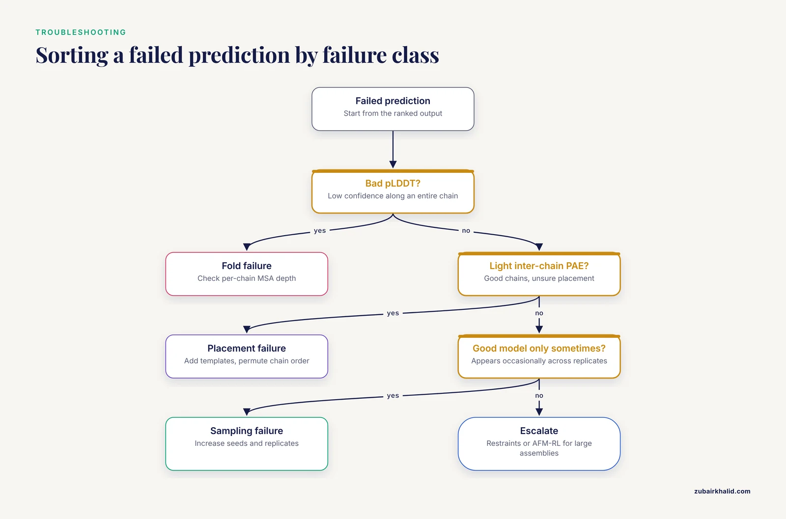
The following table consolidates the failure modes reported most often in heteromer work, with the diagnostic and the fix for each.
| Symptom | Likely cause | Fix | |
|---|---|---|---|
| , | , | , | |
| Output PDB contains one chain only | Monomer preset used, or ColabFold treated each record as a separate monomer job | Check the preset; use the single-record `>N | name` format for ColabFold or the multimer preset for the official pipeline |
| Out of GPU memory on a large assembly | Total length or MSA depth exceeds memory | Reduce MSA depth for a triage pass, shorten low-complexity regions if annotated as such, or route the job to AFM-RL for six to twenty chain assemblies [14] | |
| ipTM low across every seed and model | Shallow MSAs, unfamiliar interface, or wrong stoichiometry | Check per-chain MSA depth, test alternate chain orders and copy numbers, add templates if homologous complexes exist [6] | |
| ipTM high but PAE inter-chain blocks light | Ranking metric noise on a borderline model | Read the matrix directly; require dark blocks at the contacting residues before trusting the interface | |
| Top-ranked model differs wildly between seeds | Genuine sampling ambiguity | Increase seed count, treat the model ensemble as the answer, and consider experimental restraints [12][13] | |
| One chain is fully disordered in every model | Chain may be intrinsically disordered or lack MSA signal | Verify disorder expectation independently; disordered partners will not be placed by the network meaningfully | |
| Model contradicts known crosslink distances | Network sampled the wrong state | Feed the distance data into a restraint-based pipeline such as ColabDock rather than discarding the prediction [12][13] | |
| Screen scores show no separation between test pairs and negative controls | Non-specific interface generation in the absence of real signal | Expand and randomize negative controls; score distributions need a floor [3] |
A general diagnostic principle: when a heteromer prediction fails, first determine whether the failure is in the fold, the placement, or the sampling. Fold failures show up as bad pLDDT along an entire chain. Placement failures show up as good chains with light inter-chain PAE. Sampling failures show up as good models that appear only occasionally across replicates. Each failure class has a different remedy, and applying the wrong remedy, for example adding seeds to a fold failure, wastes compute without changing the outcome.
A decision framework for borderline results
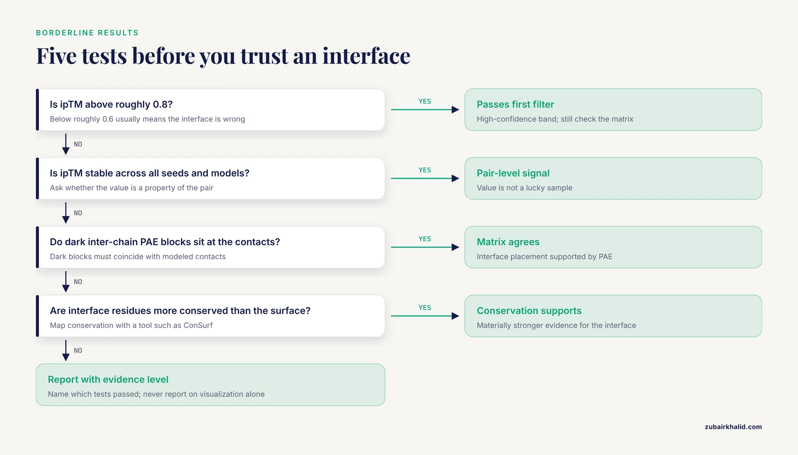
Many real heteromer predictions land in the ambiguous middle band rather than at clear accept or reject poles. A repeatable framework helps you allocate attention honestly.
Start with the ipTM bands as rough filters: above roughly 0.8 suggests a high-confidence interface, roughly 0.6 to 0.8 deserves scrutiny, and below roughly 0.6 usually means the interface is wrong or the pair does not interact this way. Then add the consistency test: collect ipTM across all your seeds and models and ask whether the value is a property of the pair or of a lucky sample. Then add the PAE test on the top models, checking that dark inter-chain structure coincides with the modeled contacts. Then add the conservation test at the interface [5]. Finally, where the stakes justify it, add the cross-platform test: run the same complex through AlphaFold3 or Chai-1 and require agreement, as done in the ComP pilin study where six candidate DNA binding modes collapsed to two that survived across AlphaFold 3, RoseTTAFold2NA, and Chai-1 [7].
Ranking evidence levels explicitly prevents the most common analytical error, which is letting a beautiful visualization of one model override a mediocre score distribution. A useful discipline is to write, for every reported model, one sentence naming which of the five tests it passed, and to never report a model on visualization alone.
For borderline pairs in a screen, the classification context matters: confidence scores can act as a rough interaction classifier, as in the peptide-protein benchmark where AF-Multimer separated interacting from non-interacting pairs with a ROC-AUC of 0.78 and a PR-AUC of 0.61, useful but far from definitive [2]. A screen-level score is a prioritization device, not a binding assay, and your downstream plan should assume a meaningful false discovery component.
Running interaction screens at scale
Screen-sized heteromer projects deserve their own workflow, because errors that are recoverable in a single prediction become systemic at scale.
Design the batch around unique chains
Organize the screen by unique chain rather than by pair. Precompute alignments per unique chain, define one template policy, and generate pairs combinatorially from the cached inputs. This is the structure underlying the AlphaPulldown2 and five-replicate AF2-Multimer protocol used across roughly two hundred protein pairs [5], and the same architecture scales up or down. Record, per pair, the exact model version, seed list, template setting, and chain order. A screen without this manifest cannot be audited later.
Build the negative control set early
The interkingdom screen study emphasized careful sequence curation and inclusion of negative controls because AFM sometimes produces plausible-looking models for pairs with no real interaction [3]. Practically, this means selecting decoy pairs drawn from the same organism or protein families as your test pairs, so the controls are matched in length and composition rather than being convenient randoms. Analyze the control distribution first: its upper tail defines your effective score floor, and any test pair scoring inside the control range should be treated as unresolved rather than positive.
Cluster before you curate
At screen scale, individual model inspection is impossible, so cluster first. The ORP-phosphatase protocol used FoldSeek-Multimer clustering alongside its scoring metrics to group similar interface solutions [5], and the Bdellovibrio work identified novel complexes by clustering analysis combined with AFM predictions [4]. Clustering turns hundreds of models into a handful of interface families, and curation effort then concentrates on one representative per family, which is where the manual judgment belongs.
Interpret screen hits as ranked hypotheses
Because ipTM values are influenced by assembly size and MSA depth, cross-comparing absolute scores across a heterogeneous screen is unsafe. Within families of comparable pairs, rankings are more meaningful. The output of a screen should therefore be a ranked shortlist with per-pair evidence summaries, not a binary hit list, and the shortlist should be sized to what your validation pipeline, whether pulldown assays or mutagenesis, can actually absorb.
Special case: peptide heteromers step by step
Short peptide partners are the classic hard case, and they recur constantly in signaling and modification biology. The published performance baseline is a median DockQ of 0.47 across 112 complexes, with AF-Multimer providing the best separation of interacting from non-interacting pairs among benchmarked methods [2], which places peptides firmly in the "worth attempting, but only with the right protocol" category.
The core problem is alignment starvation: peptides have little or no MSA, so the network leans on general interface priors and on the receptor chain's alignment. Benchmark analyses show that both the protein and peptide unpaired MSAs contribute to accuracy while the paired coevolutionary signal contributes weakly, so do not invest in elaborate pairing for peptide jobs [8][9]. What moves the needle instead is sampling diversity and, where available, forced sampling strategies that constrain the peptide during part of the prediction and improve docking outcomes [2].
A concrete protocol that follows from this evidence: run the receptor and peptide as a standard two-chain job with five models and a raised seed count; inspect the ranked ipTM distribution; if the top models disagree on where the peptide binds, treat the ensemble as competing hypotheses and rank them against any available experimental footprint; if the peptide is systematically unfolded or detached in every sample, escalate to a forced sampling protocol rather than adding more seeds to the same configuration. Throughout, remember that AF-Multimer excelled in template-based mode for this problem class [6], so if any homologous peptide-protein complex exists in the PDB, enabling templates is likely your single biggest accuracy lever.
Special case: antibody-antigen and conformational-change targets
Two target classes deserve explicit expectation management. Antibody-antigen prediction is the weakest performance class for AF-Multimer, succeeding in roughly one in five benchmark cases [1], because antibodies pair shallow germline-derived evolutionary signal with interface geometry that varies per clone. The published rescue route is AlphaRED, which uses AlphaFold as a template generator and pLDDT as a flexibility estimator, then applies physics-based replica exchange docking; it converted 63% of benchmark targets into CAPRI acceptable or better predictions, including many AF-Multimer failures, and roughly doubled antibody-antigen success relative to AFM alone [1]. If your target is an antibody-antigen pair, budget for that pipeline rather than iterating endlessly on seeds.
Conformational-change targets are subtler, because the failure is not visible as failure. AlphaFold-family models tend to default to one dominant conformational state, and the mitochondrial ADP/ATP carrier example is instructive: both AF2 and AF3 biased toward the cytoplasmic-facing state, while a ColabFold implementation could recover the matrix-facing state, meaning implementation details alone changed which state was captured [10]. For a heteromer whose biology involves a state transition, a single confident model is evidence about one state, not about the transition. Run multiple implementations or sampling regimes and treat state diversity across them as part of the result.
Comparing the three routes in detail
The earlier section introduced the three routes; the following comparison makes the selection criteria explicit for heteromer work specifically.
| Dimension | AlphaFold server | ColabFold | Official pipeline |
|---|---|---|---|
| , | , | , | , |
| Input types | Proteins, nucleic acids, ligands, modifications | Protein chains | Protein chains |
| Seed and replicate control | Not user-controlled | Full control via -num-seeds and models | Full control via -num_multimer_predictions_per_model and seed options |
| Batch screening | One job at a time | Batch mode with cached MSAs | Batch via scripting over FASTA files |
| Custom databases and templates | No | Partial, with local MSA databases | Full |
| Reproducibility for publication | Limited by server-side changes | High, version-pinned locally | Highest, exact DeepMind behavior |
| Hardware needed | None | NVIDIA GPU, practical minimum 24 GB for two-chain jobs | NVIDIA GPU plus database storage |
| Commercial use | Non-commercial terms apply | Check license terms of components | Check license terms of components |
A reasonable division of labor: prototype on the server when a complex includes ligands or nucleic acids and the question is exploratory; run screens and seed sweeps in ColabFold; reserve the official pipeline for publication-grade runs where exact version and parameter provenance matter, or where cluster integration is required. The multi-platform verification habit cuts across all three routes: for complexes involving DNA or unusual chemistry, agreement between independent systems was decisive in filtering six candidate binding modes down to two robust ones [7].
Common misconceptions, corrected one by one
Misconception: a high pLDDT model of a complex proves the interaction. pLDDT scores each residue's local geometry within its chain. A heteromer model can have every residue above the highest confidence band while the interface is pure fiction, because pLDDT never evaluates inter-chain placement. Interface claims require ipTM, inter-chain PAE, and replication.
Misconception: the top-ranked model is the answer and the rest are noise. The ranker is a useful heuristic, but for borderline interfaces the ensemble is the real result. A spread of plausible interfaces across seeds is a finding, and forcing a single narrative onto it misrepresents the evidence. The five-replicate design used in screening exists precisely because single predictions are samples [5].
Misconception: ipTM is comparable across all complexes. Assembly size and MSA depth shift ipTM, so a 0.65 on a six-chain assembly is not the same evidence as a 0.65 on a compact dimer. Within-family comparisons and control distributions are the sound ground for rankings.
Misconception: more recycles will fix a bad interface. Recycling refines geometry the network has already engaged with. If the inter-chain PAE is uniformly light across models, the problem is information, not refinement, and the remedy is MSAs, templates, or restraints, not another recycle.
Misconception: a failed prediction means the proteins do not interact. Failure modes include shallow MSA, unfamiliar interface topology, and wrong stoichiometry. Negative prediction is only defensible when controls establish a score floor and the pair still falls inside it [3]. Conversely, training bias for previously seen interface types means confident models of novel targets need extra scrutiny, not less [8][9].
Misconception: AlphaFold-Multimer is superseded and no longer worth running. Systematic comparisons show a mixed picture: on the protein-peptide benchmark, AlphaFold3 produced high-quality structures for more individual proteins, but the median accuracy was not better than AF-Multimer with a large model pool, and AF-Multimer excelled with templates [6]. Meanwhile, the surrounding ecosystem, from AFM-RL for large assemblies [14] to split-and-merge pre-training that surpassed both AF-Multimer and AF3 on several CASP15 dimer targets after fine-tuning [17], continues to build directly on the Multimer framework. Knowing Multimer deeply remains a good investment.
From model to experiment: designing the validation loop
The final stage of a heteromer project is converting a ranked model into an experimentally testable claim, and the design of this loop should start from the model's own confidence structure.
Prioritizing mutations
Interface residues for mutagenesis should come from the intersection of three signals: residues with low inter-chain PAE in the top-ranked models across replicates, residues conserved across the chain's alignment [5], and residues whose mutation would disrupt a chemically specific contact rather than merely bury hydrophobic surface. A residue that scores on all three is a far better single-mutant candidate than the residue with the single darkest PAE value. Design mutants that disrupt the interface without destabilizing the fold, and interpret a loss-of-function pulldown together with an expression or folding control, because a mutation that breaks the fold will mimic a break in the interface.
Folding in sparse experimental data
When orthogonal data exists, the strongest move is to feed it back into prediction rather than using it only as a post-hoc filter. Covalent labeling mass spectrometry data integrated with AlphaFold models in Rosetta docking distinguished native-like from non-native models that unguided modeling could not resolve [11]. ColabDock inverts the AlphaFold prediction network to incorporate sparse restraints such as NMR chemical shift perturbations or covalent labeling without retraining, and outperformed HADDOCK and ClusPro on those restraint types [12][13]. Both approaches assume you have the data; the planning insight is that a modest crosslinking or labeling experiment, sized to produce a handful of distance restraints, can rescue a borderline computational result that no amount of additional sampling would fix.
Closing the design loop
The machinery runs both directions. Cyclic peptide complex offsets applied to AF-based binder hallucination produced cyclic peptide designs targeting protein-protein interfaces, validated against the native MDM2/p53 geometry among other targets [16], which illustrates how a validated heteromer interface becomes a starting point for designed binders. And on the methods side, the CAPRI community experience showed that integrating AlphaFold into docking pipelines with enhanced sampling improved accuracy across successive rounds [15], a lesson that applies equally to an individual lab: AFM output plus deliberate, structured sampling beats AFM output alone.
What to report
For any published or internally reported heteromer model, report the model version, the number of models and seeds, the template setting, the chain order, the full ipTM and pTM distribution across replicates rather than only the top value, the inter-chain PAE status of the reported interface, and the control behavior if the model came from a screen. This reporting standard costs almost nothing to satisfy while you work and is nearly impossible to reconstruct afterward. It is also what allows a colleague, or you in two years, to distinguish a well-supported interface from a lucky sample.
Extending your toolkit: what to learn next
Once the core heteromer workflow is routine, four extensions repay the investment. First, learn the pairwise-to-assembly paradigm through AFM-RL if large assemblies are on your roadmap, since it covers six to twenty chain complexes that defeat single-pass prediction [14]. Second, learn a restraint-aware pipeline such as ColabDock, because most interesting biological systems eventually produce some sparse experimental data, and knowing how to fold it into prediction changes what experiments you order [12][13]. Third, follow the conformational-state literature for your protein families, since the state-bias findings [10] imply that routine practice should include state-diverse sampling rather than single-state reporting. Fourth, keep a running cross-platform check on your problem class: the relative standing of AF-Multimer, AlphaFold3, Chai-1, and newer systems shifts with each benchmark, and the consensus-across-platforms habit [7] is robust to those shifts in a way that loyalty to any single system is not.
The unifying thread across all of this is that AlphaFold-Multimer for heteromeric complexes is strongest when treated as a sampling and evidence-weighing system rather than an oracle. The commands are simple; the discipline around stoichiometry, replication, matrix reading, and controls is what turns a plausible picture into a defensible biological claim.
Frequently Asked Questions
Can AlphaFold-Multimer predict heteromeric complexes or only identical chains?
It predicts both. Heteromers, where each chain has a different sequence, work the same way as homo-oligomers at the input level, with each chain supplied as its own sequence, though accuracy for heteromers depends heavily on MSA depth and interface familiarity.
What ipTM score should I trust?
A practical community threshold is ipTM above roughly 0.8 for high-confidence interfaces and below roughly 0.6 for likely incorrect ones, with the middle band requiring case-by-case judgment. Always interpret ipTM together with the inter-chain PAE matrix rather than in isolation.
How do I format a FASTA file for a multi-chain prediction?
For ColabFold batch, put all chains in a single record with the chain count in the header, one sequence per line, like >2|my_complex. For the official AlphaFold pipeline, provide one FASTA record per chain in the same file and run with the multimer preset.
Should I use the AlphaFold server or a local installation?
Use the server for quick single predictions and when you need ligands or nucleic acids included, since it supports those entity types. Install ColabFold or the official pipeline locally when you need batch processing, seed control, custom parameters, or jobs that exceed the server's size limits, which are published on the server's help pages.
Why do my antibody-antigen predictions fail?
Antibody-antigen interfaces are among the hardest cases because binding involves conformational changes and shallow evolutionary signal, and AF-Multimer succeeds in only about one in five such targets in benchmarks. Use docking-based rescue methods such as replica exchange approaches that start from AF templates, or add experimental restraints.
How many seeds and recycles do I need?
For straightforward heteromers, five models with three recycles is a reasonable default. For difficult or borderline interfaces, five seeds per model, giving 25 samples, plus five replicates if you are screening, gives a ranking you can trust more than any single run.
How does AlphaFold-Multimer compare with AlphaFold3?
AlphaFold3 handles proteins, nucleic acids, ligands, and modifications in one system and often produces good models, but head-to-head benchmarks on some problem classes show AF-Multimer with a large model pool still matching or beating it, especially with templates available. The sound practice is to run both on important targets and require consensus.
Can AlphaFold-Multimer predict protein-peptide complexes?
Yes, and it is competitive, with a median DockQ around 0.47 across a 112-complex benchmark and the best ability among tested methods to separate interacting from non-interacting pairs. Peptides lack deep MSAs, so forced sampling and multiple seeds materially improve peptide results.
Sources
- Reliable protein-protein docking with AlphaFold, Rosetta, and replica-exchange
- Improving peptide-protein docking with AlphaFold-Multimer using forced sampling
- Using AlphaFold Multimer to discover interkingdom protein-protein interactions
- Using AlphaFold-Multimer to study novel protein-protein interactions of predation essential hypothetical proteins in Bdellovibrio
- AlphaFold-driven discovery of oxysterol-binding protein-related protein-phosphoinositide 3-, 4-, and 5-phosphatase interactions using new generation confidence scores
- Comprehensive Evaluation of AlphaFold-Multimer, AlphaFold3 and ColabFold, and Scoring Functions in Predicting Protein-Peptide Complex Structures
- Two different and robustly modeled DNA binding modes of Competence Protein ComP - systematic modeling with AlphaFold 3, RoseTTAFold2NA, Chai-1 and re-docking in HADDOCK
- How AlphaFold and related models predict protein-peptide complex structures
- Training bias and sequence alignments shape protein-peptide docking by AlphaFold and related methods
- Modeling the different conformations of the human mitochondrial ADP/ATP carrier using AlphaFold and molecular dynamics simulations of the protein-ligand complexes
- Protein complex prediction using Rosetta, AlphaFold, and mass spectrometry covalent labeling
- Integrated structure prediction of protein-protein docking with experimental restraints using ColabDock
- ColabDock: inverting AlphaFold structure prediction model for protein-protein docking with experimental restraints
- AFM-RL: Large Protein Complex Docking Using AlphaFold-Multimer and Reinforcement Learning
- Protein Complex Structure Prediction With AlphaFold-Enhanced HDOCK in CAPRI Rounds 47-55.
- Design of Cyclic Peptides Targeting Protein-Protein Interactions Using AlphaFold
- Improving protein and protein interactions using pseudo-dimers derived from monomeric proteins