How to Filter AlphaFold Models by Confidence: A Practical Workflow
By Dr. Zubair Khalid, DVM, MS, PhD ·

AlphaFold gives you two different promises in one output. Local metrics such as pLDDT tell you whether each residue's backbone is placed correctly, while pairwise and interface metrics such as PAE and ipTM tell you whether domains and separate chains are positioned correctly relative to each other, and the two classes of metrics can disagree completely on the same model.
The rule of thumb that follows from that difference is simple. For a single folded chain, keep residues and regions above a pLDDT of 70 and treat everything below 50 as decoration rather than structure [1]. For a complex of two or more chains, never accept a single model on the default ranking alone. Generate an ensemble with different random seeds, rank by interface confidence, inspect the predicted aligned error between chains, and then validate the survivors against any experimental data you can get. This article walks through both situations with concrete cutoffs, code you can paste, worked scenarios, and the failure modes that catch experienced users as often as beginners.
The confidence metrics you will actually use
Before filtering anything, you need to know exactly what each number claims to measure. AlphaFold's own quality assessment is built on the predicted local distance difference test (pLDDT), a per amino acid confidence score, and most downstream selection work either extends that score or corrects for its blind spots [2].
pLDDT, the per-residue score
pLDDT is a number between 0 and 100 assigned to every residue. It estimates the fraction of nearby backbone atoms that the model expects to place correctly. In the PDB files produced by AlphaFold and by the AlphaFold Protein Structure Database, pLDDT is written into the B-factor column, which means you can read it with any structure parser or even a one-line shell command.
The widely used interpretation bands are:
| pLDDT band | Interpretation | Typical action |
|---|---|---|
| 90 to 100 | Very high confidence, backbone geometry usually highly accurate | Trust for modeling, docking, and restraint generation |
| 70 to 90 | Confident backbone, side chains and exact rotamers less certain | Trust the fold, be careful with fine detail |
| 50 to 70 | Low confidence, possible but unreliable | Inspect manually, treat as hypothesis |
| Below 50 | Very low confidence, often intrinsically disordered | Do not interpret, crop or model separately |
The pLDDT of 70 is the standard rule-of-thumb cutoff for high confidence in the eukaryotic predictions distributed through the AlphaFold Protein Structure Database, and a large survey of the human proteome found that many predictions contain extensive regions below that line [1].
Low pLDDT regions are not all the same. A detailed categorization divides them into three behavior modes. Near-predictive regions resemble folded protein and can approach an accurate prediction. Pseudostructure shows an intermediate pattern with a misleading appearance of isolated, badly formed secondary structure elements. Barbed wire is extremely unprotein-like, with wide looping coils, an absence of packing contacts, and numerous validation outliers, and it carries no predictive value at all [1]. A model with a low average pLDDT can therefore still contain a perfectly usable folded core sitting next to a barbed wire tail, and your filter should be region aware rather than model average aware.
PAE, the pairwise matrix
The predicted aligned error (PAE) is a square matrix with one row and column per residue, reported in Angstroms. Entry (i, j) estimates the expected position error of residue j when the structure is aligned on residue i. Where pLDDT says how well a residue is placed, PAE says how confidently the model knows where two residues sit relative to each other.
You use PAE in two ways. Within a chain, block structure in the PAE matrix reveals domains: residues inside one domain show mutual errors of a few Angstroms, residues in different domains show errors of 10 Angstroms or more, and the boundary between blocks tells you where flexible linkers live. Between chains in a complex, the off-diagonal blocks report how confidently the two chains are packed against each other. A low interchain PAE block means the model places the interface with conviction, which matters far more than the individual chains' pLDDT values.
pTM and ipTM
The predicted template modeling score (pTM) and its interface counterpart ipTM are numbers between 0 and 1 that estimate template-modeling quality, meaning the expected fraction of structurally equivalent residues, either within a chain (pTM) or across the interface of a complex (ipTM). The AlphaFold-Multimer literature treats an ipTM near 0.8 as a strong interface and values below roughly 0.6 as likely failed interfaces, and multimer runs are typically ranked by a composite of ipTM and pTM. Treat those cutoffs as calibrated for generic protein complexes. They transfer poorly to antibody-antigen pairs and other interfaces with weak coevolutionary signal, a point examined in detail below [3].
ranking_score and model rank
AlphaFold3 and its server report a ranking_score, and local pipelines produce a rank ordering (rank_0, rank_1, and so on). The rank is a useful default sort but is not a statement of truth. A CAPRI assessment of AlphaFold-based docking rounds found that a highly accurate model for one antibody-MHC target ranked low, so an honest workflow keeps more than the top ranked candidate and rescores the pool [4].
Where AlphaFold models come from, and what that means for filtering
Your model selection confidence strategy depends on where the models originate, because different sources give you different amounts of ensemble data to filter.
The AlphaFold Protein Structure Database. Maintained by EMBL-EBI, this resource provides one precomputed model for nearly every cataloged protein sequence. There is no ensemble here, so filtering means cropping per-residue rather than choosing among models. Download the structure with its pLDDT values in the B-factor column, and the associated PAE matrix, and work region by region.
The AlphaFold Server. The AlphaFold Server is Google DeepMind's official web interface for AlphaFold3. You paste protein sequences, nucleic acid sequences, ligands, and modifications, the server runs the prediction, and you download the coordinates together with confidence outputs including pLDDT in the B-factors, the PAE matrix, and summary scores such as ipTM, pTM, and ranking_score. The server enforces a daily job allowance and offers limited control over sampling, so treat each submission as a small ensemble of ranked models and filter on the confidence files after download. Most AlphaFold tutorial material, from the ColabFold notebooks to the official server help pages, now centers on exactly this download-and-filter step.
Local and notebook runs. Running AlphaFold2 through ColabFold, or AlphaFold3 through licensed local installations, gives you real sampling control: multiple models per sequence, multiple random seeds, template on or off, and adjustable recycling. This is the setting where model selection confidence actually becomes a ranking problem, because you have a pool of dozens of decoys to filter rather than one or five.
Side-by-side comparison of the main filtering options
This table is the core of the workflow. Each option is expanded in the sections that follow.
| Option | What it measures | Best for | Pros | Cons |
|---|---|---|---|---|
| pLDDT cutoff (70, crop below 50) | Per-residue local accuracy | Single chains, domain extraction, trimming tails | Simple, per-residue, built into every PDB | Blind to interface quality, inflated for memorized folds |
| PAE inspection | Relative position error, in Angstroms, residue to residue | Domain boundaries, interface ordering, chain packing | Localizes exactly which contacts are trusted | Needs scripted or visual interpretation, no single number |
| ipTM cutoff (near 0.8 strong, below 0.6 suspect) | Interface accuracy of a complex | First-pass triage of multimer pools | One interpretable number per model | Poor discrimination for antibody-antigen and low-coevolution targets [3] |
| pTM | Per-chain fold quality in a complex | Checking each chain folds correctly | Catches folded-part failures that ipTM hides | Says nothing about the interface |
| Default model rank / ranking_score | Model's own composite score | Initial ordering of a pool | Zero effort, calibrated on benchmarks | Accurate models can rank low [4], weak for hard targets |
| Ensemble consistency across seeds | Reproducibility of the prediction | Complexes, hard targets | Separates convergent solutions from lucky draws | Costs compute, needs clustering |
| External rescoring (learned rankers, docking scores, validation servers) | Agreement with independent evidence or trained priors | Antibody-antigen, drug discovery pipelines | Recovers models the native metrics miss | Method-specific bias, extra setup |
| Experimental data agreement (SAXS, NMR CSP, crosslinking) | Agreement with measurements | Any model destined for publication | The strongest filter that exists | Requires data, slowest option |
The step-by-step workflow
This section is the practical answer to how to filter AlphaFold models by confidence, written so you can execute it end to end.
Step 1: Define what the model must be right about
A model used to pick a docking box needs an accurate pocket. A model used to argue about an interface needs accurate chain placement. A model used to design mutations in a folded domain needs that domain only. Write the requirement down first, because it decides which metric leads and which cutoffs apply. In structure-based drug discovery work, prediction confidence and accuracy vary considerably by target and by region within a target, so the same protein can be excellent at the active site and unreliable at the allosteric cleft [5].
Step 2: Extract every metric from every model
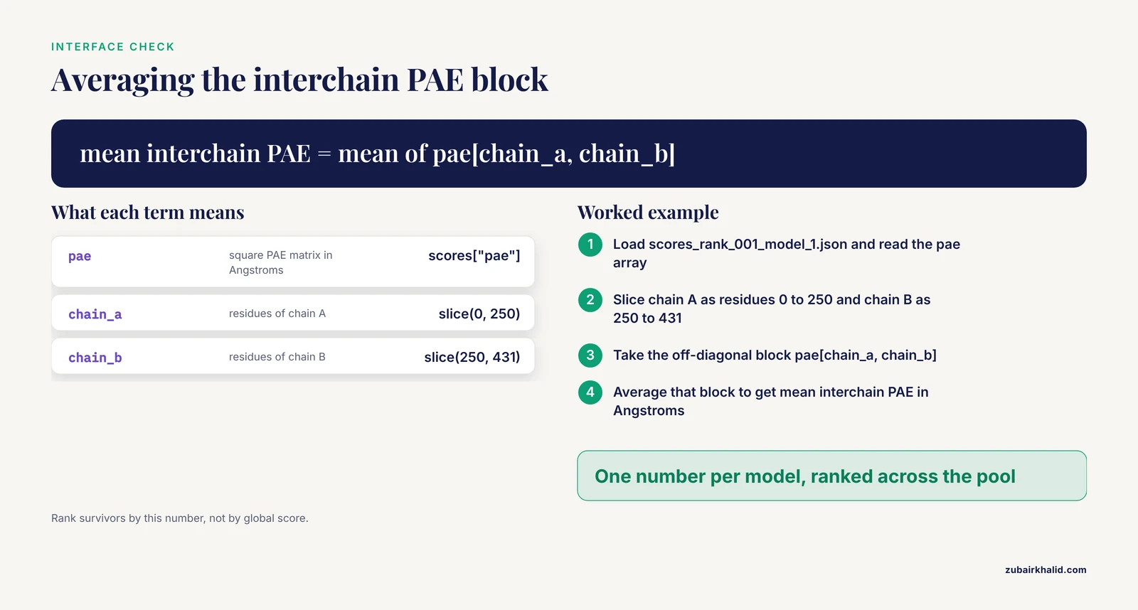
For monomers from the database or from a local run, pull per-residue pLDDT from the B-factor column:
from Bio.PDB import PDBParser
import numpy as np

model = PDBParser(QUIET=True).get_structure("af", "rank_001_model_1.pdb")
plddt = np.array([res["CA"].bfactor for res in model.get_residues() if "CA" in res])

print("mean pLDDT:", round(float(plddt.mean()), 1))
print("fraction above 70:", round(float((plddt >= 70).mean()), 3))
core = np.where(plddt >= 70)
print("longest confident stretch:", core.min() + 1, "to", core.max() + 1)
A quick shell check does the same job when Biopython is not handy, reading pLDDT from column 11 of ATOM records:
awk '$1=="ATOM" && $3=="CA" {s+=$11; n+=1} END {print s/n}' rank_001_model_1.pdbFor multimer runs, load the scores file that ColabFold writes alongside each model, which carries the PAE matrix and the summary scores:
import json
import numpy as np

with open("scores_rank_001_model_1.json") as handle:
    scores = json.load(handle)

print("ipTM:", round(scores["iptm"], 3))
print("pTM:", round(scores["ptm"], 3))

pae = np.array(scores["pae"])
chain_a = slice(0, 250)      # residue count of chain A
chain_b = slice(250, 431)    # residue count of chain B

inter = pae[chain_a, chain_b]
print("mean interchain PAE (A):", round(float(inter.mean()), 2))
For AlphaFold Server output, the downloaded archive includes a summary confidences file with the same headline numbers, so the same filtering logic applies regardless of where the prediction ran.
Step 3: Filter single chains region by region
Apply the region bands from the table above. Keep everything at pLDDT 70 and above for structural interpretation, flag 50 to 70 for manual inspection, and crop or separately handle everything below 50. Then refine with two additional checks.
First, look for coherent stretches rather than raw values. Methods grounded in topological data analysis identify contiguous amino acid stretches with consistent pLDDT behavior, which cleanly separates a reliable domain from a pseudostructured stretch, and the implementation ships in the Alphafold_analysis package of the Structural Bioinformatics Library [2].
Second, classify the low-confidence regions. If a low pLDDT tail corresponds to an annotated disordered region, cropping it is safe and standard. If it forms a pseudostructure, a pattern with a misleading appearance of secondary structure elements, it will look like a helix bundle in a viewer while meaning nothing. The categorization work connecting these modes to MobiDB disorder annotations and signal peptides found that barbed wire and pseudostructure track many disorder measures, while near-predictive regions associate with conditionally folding segments [1]. A Phenix tool now implements this annotation and visual markup directly on the prediction, which is the fastest way to make the call.
Finally, run independent structure validation on the confident core. A published modeling study of a viral polymerase used Verify3D, PROCHECK, and ERRAT alongside the confidence scores to confirm the predicted NS5 model before any docking, with pLDDT values approaching 90 and a pTM of 0.8 [6]. Comparative quality assessments of AlphaFold against homology modeling report that although AlphaFold produces high-quality structures, high-confidence parts are sometimes observed to disagree with experimental data, which is exactly the situation those validation servers are designed to expose [7].
Step 4: Filter complexes with ensembles, not single models
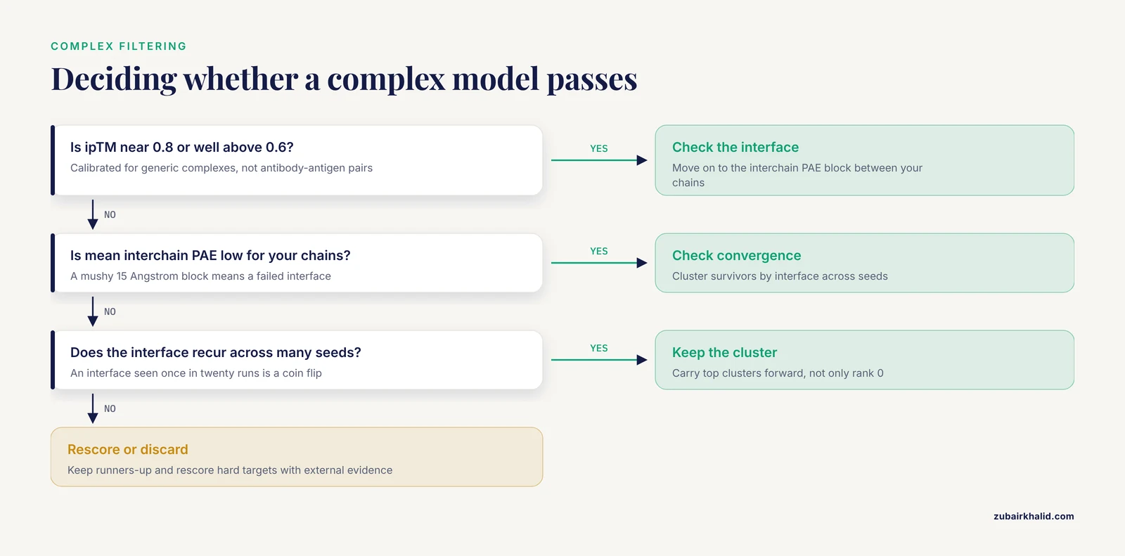
For anything with more than one chain, the workflow changes fundamentally.
- Generate an ensemble. Run at least five models (the ColabFold default) and, for hard targets, repeat across several random seeds. The point is not to find the best single run but to see which solutions recur.
- Triage with ipTM. Discard models with ipTM far below your passing threshold before anything else. For generic complexes, values near 0.8 and above indicate a strong interface while values below about 0.6 indicate a probable failure, per the AlphaFold-Multimer calibration.
- Inspect the interchain PAE block. Rank the survivors by mean interchain PAE between the chains you care about, not by global score. A model with excellent chain pLDDT and a mushy 15 Angstrom interchain PAE block is a failed interface wearing good clothes.
- Check convergence. Cluster the surviving models by interface. Interfaces that appear across many seeds deserve trust. An interface that appears exactly once in twenty runs is a coin flip, whatever its ipTM says.
- Keep the runners-up. Because accurate models can rank low [4], carry at least the top few clusters forward rather than only the top rank.
This pipeline is what made large-scale screens tractable. A benchmark of AlphaFold2 and AlphaFold3 on 6,782 pathogen-human protein interactions found that accurate models could be retrieved when ranking by modeling confidence, despite overall low performance, and 803 higher-confidence models emerged from that screen [8]. The yield is modest and that is the point. Confidence-based filtering at scale is a precision instrument, not a guarantee of a hit for every pair.
Step 5: Rescore hard targets with external evidence
Some target classes defeat the native metrics outright. Antibody-antigen complexes are the canonical case, because they lack strong coevolutionary information and AlphaFold3 often generates accurate predictions but fails to reliably distinguish them from the much larger set of incorrect ones [3]. Three external strategies are in mainstream use.
Learned rankers. ABAG-Rank is a deep neural network built on a permutation-invariant DeepSets architecture that takes variable-sized ensembles of structural decoys and scores interface quality using simple geometric descriptors together with AlphaFold confidence scores, without intensive physics-based calculations. Trained on a redundancy-reduced set of all known antibody-antigen complexes, it significantly outperforms AF3 internal scoring for this task [3]. If you work on antibodies, this class of tool is the single biggest upgrade available to your selection step.
Experimental restraints. When you have NMR chemical shift perturbation data, the CSP_Rank approach combines AlphaFold2 enhanced sampling with a Bayesian conformational selection process driven by the experimental perturbations and AF2 confidence metrics. Across a curated set of 108 protein-peptide complexes from the Biological Magnetic Resonance Data Bank, enhanced sampling followed by data-guided selection routinely produced ensembles with improved agreement with the NMR observables compared with plain AF2 output [9]. A separate protocol describes selecting reliable AlphaFold predictions, extracting atom distances from them, and converting those distances into high-confidence restraints that reduce NOE assignment ambiguity during solution NMR structure determination [10].
Physical and integrative evidence. Small-angle X-ray scattering is the workhorse check for flexible proteins. In a careful comparison against curated monodisperse entries from the Small-Angle Scattering Biological Data Bank, three cases showed clear evidence that a single AlphaFold structure could not account for the experimental data, while excellent agreement was found with ensemble models built by treating the low-confidence linkers as flexible [11]. The companion website SAXS-A-FOLD automates this: you upload your scattering profile and an AlphaFold structure, the site color-codes the model by confidence level, proposes flexible regions automatically, and generates an optimized ensemble against your data [12].
Step 6: Record your decision trail
Whatever passes your filter, log the AlphaFold version, the number of models and seeds, the metric distributions of the rejected and accepted pools, and the validation steps applied. Selection confidence is only reproducible if the ensemble and the criteria are part of the record. A reviewer asking "why this model and not rank 0" should be answerable from your own files.
Four worked scenarios
Scenario 1: A single-chain enzyme target for docking
You need a human enzyme for virtual screening. Download the AlphaFold Database model, compute the pLDDT profile, and find the active site sits in a 90-plus stretch while a 60-residue C-terminal tail sits below 50. Crop the tail, then run Verify3D, PROCHECK, and ERRAT on the core as an independent check, mirroring the validation stack used before structure-based lead identification on a flaviviral polymerase model [6]. For docking campaigns specifically, the review literature on AlphaFold-driven structure-based drug discovery treats exactly this split between confident cores and variable regions as the central practical concern, affecting target preparation, docking, and downstream interpretation [5]. One refinement: comparative work on the P2X7 receptor assessed confidence levels specifically at orthosteric and allosteric binding sites across AF2, AF3, and homology models before docking, because a global average tells you nothing about whether the pocket you are about to dock into is real [13].
Scenario 2: An antibody-antigen complex
You predict 25 models across several seeds for an antibody bound to its antigen. ipTM values cluster around 0.65, which would be marginal for a generic complex, and the ranking favors one interface. Do not stop there. This is precisely the regime where AF3's internal scoring struggles, since the method often generates accurate predictions but cannot reliably separate them from incorrect ones in the pool [3]. Run an antibody-specific ranker such as ABAG-Rank over the full ensemble, keep the top clusters from that rescoring, and check whether the native ranking and the learned ranking agree. The CAPRI assessment adds a second caution drawn from real blind predictions: a highly accurate antibody-MHC model ranked low, so the interface clusters discarded early on rank alone may contain your answer [4].
Scenario 3: A multidomain protein with flexible linkers for SAXS
You have a two-domain protein with a linker that predicts at pLDDT in the 40s. Crop at the domain boundaries using the PAE block structure rather than an arbitrary residue count, verify the linker region falls into the pseudostructure or barbed wire categories rather than near-predictive [1], and then test the single rigid model against your SAXS curve. If the fit fails while individual domains are high confidence, the failure is the linkers, exactly as demonstrated on curated SASBDB entries where ensemble models built from high-confidence domains with flexible linkers reproduced the data that single structures could not [11]. The SAXS-A-FOLD web service makes this loop fast by proposing flexible regions from the confidence coloring automatically [12].
Scenario 4: A host-pathogen interaction screen
You want structural models for hundreds of predicted pathogen-human protein interactions. Predict all pairs, rank strictly by modeling confidence, and set your expectations from the published benchmark: 803 higher-confidence models out of 6,782 predicted interactions, with accurate models recoverable by that ranking [8]. Accept the low yield as informative rather than fighting it with looser cutoffs, because loosening the threshold admits mostly incorrect interfaces. If you want to increase yield upstream instead, guiding predictions toward likely interacting fragments using curated high-confidence interface types is the documented route: of 1,129 predicted domain-domain interactions flagged from a high-confidence reference set, 604 yielded confident AlphaFold models, and for 47 percent of the predictions no confident structural model could be obtained [14].
Alphafold model selection confidence options: pros and cons
Readers searching for the best alphafold model selection confidence usually want the honest trade-off list. Here it is, option by option.
pLDDT-only filtering. Pros: trivial to compute, universally available, per-residue resolution, well-calibrated for folded domains. Cons: completely blind to interchain geometry, averages hide domain structure, and the score can be high for a fold the network has essentially memorized [15].
ipTM-only filtering for complexes. Pros: one number, fast triage of large pools, works reasonably on generic complexes. Cons: the calibration was learned on typical coevolving complexes and degrades on antibody-antigen pairs, where learned rankers outperform AF3 internal scoring [3]. A single ipTM also hides which side of the interface is the problem.
PAE-based inspection. Pros: the most informative metric available, localizes trust to specific residue pairs and interfaces. Cons: no single pass-or-fail number, requires scripting or careful viewer work, and interchain PAE thresholds must be re-derived per system class.
Ensemble consistency. Pros: the only purely computational check that distinguishes a reproducible solution from a lucky draw, and the approach that rescued fold-switch and SAXS studies from single-model thinking. Cons: multiplies compute cost, needs clustering infrastructure, and consistency across seeds still cannot rescue targets where the network systematically ignores the input sequence (see the limitations section).
External learned rankers. Pros: measurably outperform native scoring on the hardest target class, antibody-antigen [3], and incorporate geometric descriptors the native scores lack. Cons: domain-specific, adds a dependency, and inherits the biases of whatever training set it learned from.
Experimental data-guided selection. Pros: the closest thing to ground truth in the loop, demonstrated to improve agreement over AF2 output alone when NMR chemical shift perturbations are available [9]. Cons: requires data you may not have, and each data type (SAXS, NMR, crosslinking) constrains only part of the structure.
Pure default ranking. Pros: free, fast, the correct choice when the target is easy and the pool is homogeneous. Cons: demonstrably capable of burying an accurate model low in the pool [4], and ranking_score is a composite that cannot be decomposed into the specific contact you care about.
Common Mistakes and Limitations
Mistake 1: Reading pLDDT as a guarantee of correctness. Confidence metrics are the model's self-assessment, and that self-assessment has documented blind spots. In a systematic adversarial evaluation across 200 proteins, predicted structures stayed invariant to mutations of up to 40 percent of residues, including deliberately destabilizing substitutions, and confidence metrics selected the most accurate structure at most 35 percent of the time in that setting, correlating with the quality of the best training-set template rather than with the mutated target [15]. High pLDDT on a heavily mutated sequence is a warning, not a certificate.
Mistake 2: Trusting rank 1 by default. Two independent lines of evidence converge here. The CAPRI assessment documented a highly accurate model that ranked low [4]. Separately, for fold-switching proteins, AF2's confidence metrics selected against models consistent with the experimentally determined alternative conformations and failed to discriminate between low and high energy states [16]. Keep multiple ranked models and rescore.
Mistake 3: Applying monomer cutoffs to complexes. The pLDDT 70 rule answers a different question than "is this interface real." A complex with beautiful per-chain pLDDT and a 15 Angstrom interchain PAE block has failed, and only PAE and ipTM can see it.
Mistake 4: Assuming low pLDDT means useless. The near-predictive mode within low-pLDDT regions can be nearly an accurate prediction and corresponds to conditionally folding regions, so automatic cropping of everything below 70 throws away usable information in some proteins [1]. Classify before you crop.
Mistake 5: Ignoring what the model cannot see. AlphaFold is a weak predictor of fold switching, achieving a 35 percent success rate for fold switchers likely present in its training sets across hundreds of thousands of models, and capturing only one of seven experimentally confirmed fold switchers outside the training sets despite extensive sampling [16]. If your protein has an documented alternative fold, confidence filtering cannot select for the alternative because the ensemble rarely contains it.
Mistake 6: Skipping experimental validation entirely. High-confidence regions sometimes disagree with experimental data [7], and single predicted structures demonstrably fail to fit SAXS data from flexible proteins [11]. If the model supports a claim in a paper, at least one orthogonal check belongs in the pipeline.
Mistake 7: Mixing versions silently. AF2 and AF3 rank and score differently, and their relative performance flips by task. In a GPCR-peptide benchmark, AF2 reproduced correct binding modes in 94 percent of 67 recent complexes, surpassing both AF3 and Chai-1 on that measure [17]. Record the version and resist the assumption that the newest model wins every comparison.
Limitation, stated once. Every cutoff in this article is a heuristic calibrated on population-level benchmarks, and individual systems, especially those with unusual biology, need case-by-case judgment backed by whatever experimental data the project can generate.
Frequently Asked Questions
What pLDDT cutoff should I use for my AlphaFold model?
Use 70 as the working threshold for confident backbone, keep everything above 90 for high-precision work such as docking and restraint generation, and treat regions below 50 as lacking predictive value. The 70 line is the established rule of thumb for the database predictions, and regions below it split into near-predictive, pseudostructure, and barbed wire behaviors that deserve different handling [1].
How do I filter AlphaFold models by confidence for a protein complex?
Generate an ensemble with multiple models and seeds, discard models with ipTM well below the passing range, rank survivors by mean interchain PAE between your chains of interest, and cluster the survivors by interface to check convergence. Keep more than the top rank, because accurate models sometimes rank low [4].
Does the AlphaFold Server report confidence scores?
Yes. The AlphaFold Server, Google DeepMind's official web interface for AlphaFold3, returns structures with pLDDT in the B-factor column, a PAE matrix, and summary scores including ipTM, pTM, and ranking_score. Download those files and apply the filtering workflow above after each submission.
Is the top-ranked AlphaFold model always the best one?
No. The rank reflects the model's internal composite score, not verified accuracy. Blind assessment found highly accurate models ranked low in real targets [4], and learned rescoring methods outperform the native scores for hard target classes such as antibody-antigen complexes [3].
What is the difference between pTM and ipTM?
pTM estimates the quality of each chain's fold on its own, while ipTM estimates the quality of the interface between chains. A complex can have strong pTM values with a weak ipTM, meaning the individual chains are well predicted but their relative placement is not trustworthy. Rank multimer models primarily on ipTM and interchain PAE.
Can I trust low-confidence regions of an AlphaFold prediction?
Usually not for structure, but classify them before deleting them. Below pLDDT 70, some regions are nearly accurate near-predictive segments, others are pseudostructure with misleading secondary-structure appearance, and the rest is barbed wire with no predictive value [1]. For flexible regions connecting high-confidence domains, ensemble modeling against experimental data such as SAXS is the productive path [11].
Sources
- Categorizing prediction modes within low-pLDDT regions of AlphaFold2 structures: near-predictive, pseudostructure and barbed wire.
- Characterizing the fragmentation of AlphaFold predictions.
- ABAG-Rank: improving model selection of AlphaFold antibody-antigen complexes by learning to rank.
- AlphaFold and Docking Approaches for Antibody-Antigen and Other Targets: Insights From CAPRI Rounds 47-55.
- AlphaFold-driven structure-based drug discovery: Capabilities, benchmarks and limitations for medicinal chemistry.
- AlphaFold-driven structure-guided identification of NS5 RdRp-targeting antiviral leads against Kyasanur Forest Disease Virus.
- Quality Assessment of Selected Protein Structures Derived from Homology Modeling and AlphaFold.
- AlphaFold models of host-pathogen interactions elucidate the prevalence and structural modes of molecular mimicry.
- Integrative Modeling of Protein-Polypeptide Complexes by Bayesian Model Selection using AlphaFold and NMR Chemical Shift Perturbation Data.
- Protocol for deriving distance restraints from AlphaFold for use in solution NMR structure determination.
- AlphaFold-predicted protein structures and small-angle X-ray scattering: insights from an extended examination of selected data in the Small-Angle Scattering Biological Data Bank.
- SAXS-A-FOLD: a website for fast ensemble modeling optimizing the fit of AlphaFold or user-supplied protein structures with flexible regions to SAXS data.
- Modeling the P2X7 receptor: a comparative analysis of conventional methods and AlphaFold.
- Generation of a high confidence set of domain-domain interface types to guide protein complex structure predictions by AlphaFold.
- Adversarial Sequence Mutations in AlphaFold and ESMFold Reveal Nonphysical Structural Invariance, Confidence Failures, and Concerns for Protein Design.
- AlphaFold predictions of fold-switched conformations are driven by structure memorization.
- Deep learning in GPCR drug discovery: benchmarking the path to accurate peptide binding.