Time-Efficient Reproducible Research Workflow: A Step-by-Step Guide
By Dr. Zubair Khalid, DVM, MS, PhD ·
By the end of this guide you will be able to design a time-efficient reproducible research workflow for your own lab project, from a frozen protocol through automated data analysis to a published, rerunnable package. You will set up version control, pin a computational environment, automate a repetitive wet-lab or image-analysis bottleneck, and validate the automated method against your current manual method with numbers you can defend to a reviewer or a collaborator.
You need a laptop with Git installed, a terminal, Python or R, and either conda (for environment management) or a workflow manager such as Snakemake or the R/Bioconductor package systemPipeR. For the wet-lab steps you need your existing protocol, a stopwatch or lab timer, and a spreadsheet for tracking hands-on time.
Why Time and Reproducibility Belong in the Same Workflow
Reproducible research means that another person, or you six months from now, can rerun your experiment or analysis and obtain the same result. The usual obstacle is not intelligence or effort. It is hidden variation: a reagent lot change, a manually adjusted threshold in an imaging script, a library prep that takes two days and depends on who holds the pipette.
The encouraging finding across recent method papers is that the same interventions that save time also reduce variance. A converted manual RNA-seq library prep run on a liquid handler produced libraries similar to the manual method while cutting a 2-day assay to a 9-hour automated run for a cohort of 84 samples [1]. A co-expression pulldown assay for difficult protein-protein interactions cut out the separate purification and incubation steps, saving time precisely because the exposed-to-proteolysis window shrank, and the shorter protocol improved reproducibility as a direct consequence [2]. A standardized mouse model of carotid atherosclerosis was published explicitly to make plaque induction faster and more reproducible across laboratories without genetically modified animals [3].
Time-efficient reproducible research is therefore not two goals in tension. It is one design discipline: fewer manual steps, recorded once, executed the same way every time.
The Time-Efficient Reproducible Research Workflow, Step by Step
The seven steps below work for a sequencing project, an imaging project, or a bench assay. Do them in order. Each step produces an artifact you keep.
Step 1: Define the Question and Freeze the Protocol
Write the primary endpoint in one sentence with a number in it. "CD31-positive area fraction in rat bone defect sections" is a frozen endpoint. "Look at vascularization" is not. Studies that succeed at reproducibility usually start this way. The standardized imaging workflow for cutaneous neurofibromas in Nf1-KO mice defined macroscopic endpoints (tumor count, fluorescent surface area, fluorescence intensity) and microscopic endpoints (cell-type composition and area quantification) before building any automation [4]. The carotid ligation plus PCSK9 atherosclerosis protocol specifies dosing, diet, surgical steps, postoperative care, tissue collection, and stains (Oil Red O and Verhoeff-Van Gieson) as a fixed package so that any lab can reproduce the pathology [3].
Practical rule: if a step in your protocol cannot be read by a new student and executed without asking you a question, it is not frozen yet. Write reagent names, lot numbers, incubation times, and equipment settings into the protocol document itself.
Step 2: Put Every Protocol Under Version Control
Move your protocols, analysis scripts, and sample sheets into a Git repository. Git records every change with a timestamp and an author, and a tag marks the exact version used for a given experiment.
mkdir myproject && cd myproject
git init
mkdir protocols analysis raw_data results
git add protocols/ analysis/ README.md
git commit -m "Freeze v1.0 protocol for EXP-2026-01"
git tag v1.0
Expected output on the commit line:
[main (root-commit) a1b2c3d] Freeze v1.0 protocol for EXP-2026-01
 4 files changed, 212 insertions(+)
From now on, any protocol change is a new commit, never an edit of the old text. When a reviewer asks which protocol version produced a figure, you answer with a tag name. Raw data stays out of Git (it belongs on backed-up storage with checksums, covered in Step 7), but everything humans wrote goes in.
Step 3: Pin the Computational Environment
A reproducible analysis needs the same software versions on every run. Conda solves this in one command:
conda create -n repro-rna -c conda-forge -c bioconda r-base bioconductor-systempiper salmon fastp
conda activate repro-rna
Export the solved environment so it travels with the project:
conda env export > environment.ymlAnyone can now rebuild your exact software stack with conda env create -f environment.yml. This single file removes the most common cause of "it worked on my machine": silent updates to R packages, aligners, or system libraries between the first analysis and the reviewer's rerun.
Step 4: Automate the Wet-Lab Bottleneck
Find the step that consumes the most hands-on hours and asks the most of human attention. That step is where both your time and your reproducibility leak. Recent work quantifies the pattern:
- RNA-seq library preparation took 2 days per cohort by hand and 9 hours after conversion to an automated liquid-handler protocol, with high similarity between manual and automated libraries across 84 samples [1].
- A full-length 16S rRNA gene sequencing protocol on the Oxford Nanopore MinION was streamlined specifically to reduce labor-intensive library steps and turnaround time, and it achieved higher accuracy than a MiSeq pipeline on synthetic microbial communities [5].
- An optimized DuraClone flow cytometry workflow for TBNK subset quantification cut procedural steps by 50% and processing time by 38.6% while keeping precision coefficients of variation below 10% for all subsets [6].
- A single migration and invasion assay workflow built around an automated live-cell imager replaced fragmented manual handling with one continuous, timed, imaging-integrated protocol [7].
You do not need a robot to apply the principle. Removing centrifugation steps, eliminating a tube transfer, or batching samples identically delivers the same two benefits at smaller scale. Thepulldown assay redesign in [2] is the cleanest example: merging two protocols into one saved time because the number of steps, and therefore the number of failure points, dropped.
Track your own numbers in a spreadsheet. Log hands-on minutes per batch for one week before changing anything. That baseline is what you will compare against in Step 6.
Step 5: Build the Analysis as an End-to-End Workflow
Manual, click-through analyses are the second big leak. Each image threshold adjusted by eye, each column copied between spreadsheets, is a decision nobody can audit later. Convert the analysis into a script-driven workflow that runs start to finish.
For sequencing data in R, systemPipeR provides an extensible environment for building and running end-to-end workflows with automated report generation, a uniform interface across applications, support for both R and command-line tools on local machines and clusters, and a sample annotation file (the targets file) that handles complex experimental designs [8]. A minimal session looks like this:
library(systemPipeR)

## One row per sample in targets.txt, plus columns for condition and batch
targets <- read.delim("targets.txt", comment.char = "#")
head(targets)

## Import a stored workflow definition
WF <- importWF("rnaseq_wf.Rmd")

## Run every step, in order, with logging
WF <- runWF(WF, steps = "all")

## Generate the HTML report
WF <- renderReports(WF)
Expected console output after runWF:
Loading workflow /home/you/myproject/rnaseq_wf.RMD
Processing step wf_step_trim
Processing step wf_step_align
Processing step wf_step_count
Workflow finished. 24/24 samples processed.
Report written to ./rnaseq_wf/report/rnaseq_wf.html
For file-driven pipelines outside R, Snakemake expresses the same idea as rules:
rule all:
    input: "results/counts.csv"

rule trim:
    input: "raw/{sample}.fastq.gz"
    output: "trimmed/{sample}_trim.fastq.gz"
    shell: "fastp -i {input} -o {output}"

rule count:
    input: expand("trimmed/{sample}_trim.fastq.gz", sample=samples)
    output: "results/counts.csv"
    shell: "featureCounts -a genes.gtf -o {output} {input}"
Running snakemake executes only what is out of date, in dependency order. Re-running the whole project is one command, which is the definition of a reproducible analysis.
The same automation logic applies to image data. A dual UHPLC-HRMS metabolomics and lipidomics workflow for fecal phenotyping paired its acquisition design with an automated R-based targeted peak extraction algorithm (TaPEx) so that 360 metabolites and 132 lipids could be profiled across large cohorts without manual peak picking [9]. For image fusion, the Esmraldi workflow merged mass spectrometry imaging and MRI data using deterministic methods, and the authors noted that determinism itself guarantees reproducible results on large datasets [10]. Deterministic, parameterized, scripted: those three words describe every reproducible analysis.
Step 6: Validate the Automated Method Against the Manual Reference
Automation without validation is a liability. Before you retire the manual method, run both on the same samples and compute an agreement statistic. The literature gives you concrete targets to beat or match:
- Two independently trained Trainable Weka Segmentation classifiers for CD31-stained bone sections produced highly stable values with an overall mean coefficient of variation of 1.98%, better than the good-but-human manual retest values of 7.17% and 6.84% for the two observers, and manual assessment cost 3 minutes 17 seconds (± 1:35) per section [11].
- Automated ImageJ scripts for neurofibroma quantification reached an intraclass correlation of 1 for reproducibility, correlated strongly with manual analysis (Spearman coefficient above 0.90), and ran up to 100-fold faster [4].
- A deep learning micro-CT organ segmentation tool produced identical results on repeated runs and cut segmentation from roughly 30 minutes per mouse to about 5 minutes [12].
- A deep learning echocardiography platform for global longitudinal strain measured in real time with excellent correlation to manual reference measurements (r = 0.94) and 94% feasibility across 50 patients [13].
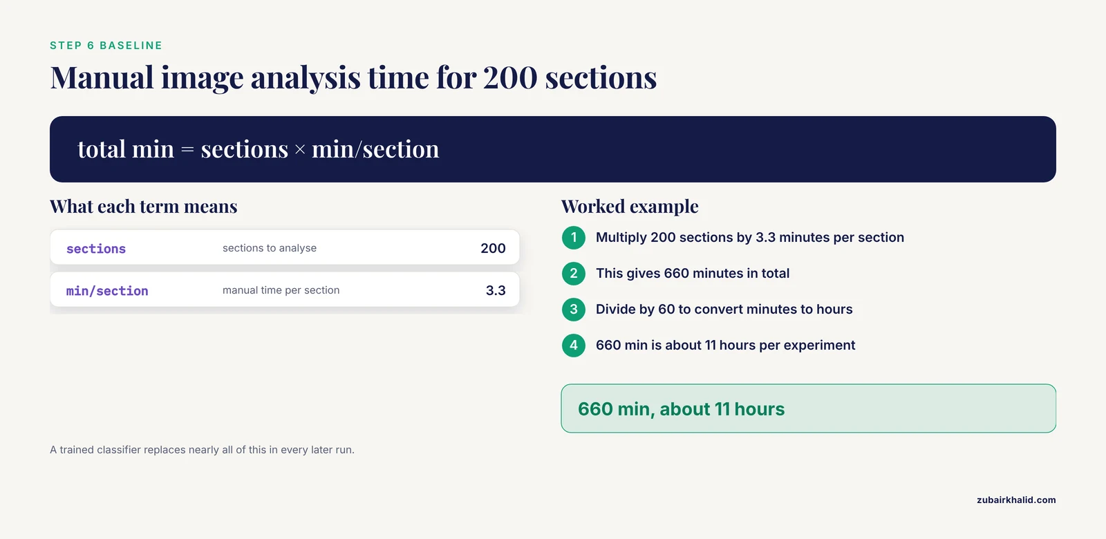
Here is the worked calculation for Step 4's baseline. Suppose your manual image analysis takes 3.3 minutes per section and you have 200 sections:
200 sections × 3.3 min/section = 660 min ≈ 11 hours of manual work per experimentAn automated classifier with a one-time training cost replaces nearly all of those 11 hours in every subsequent run, and the variance drops because the classifier applies the same rule to every pixel every time. That is the time-reproducibility dividend in one calculation.
Report three things from your validation: an agreement statistic (correlation, Bland-Altman bias, Dice coefficient, or intraclass correlation), a repeatability statistic (coefficient of variation across reruns), and a time per sample for each method. Those three numbers go into your methods section.
Step 7: Freeze the Data and Publish the Package
Checksum every raw file so corruption or accidental modification is detectable:
md5sum raw_data/*.fastq.gz > checksums.md5
md5sum -c checksums.md5
Expected output:
raw_data/sampleA.fastq.gz: OK
raw_data/sampleB.fastq.gz: OK
Then package the project for release: raw data on institutional storage or a repository, code in the tagged Git repository, environment.yml beside the code, the frozen protocol PDF, the validation report from Step 6, and the rendered workflow report. A collaborator should be able to go from raw files to your figures with two commands and no questions.
Choosing Tools: A Quick Comparison
| Bottleneck | Manual baseline | Automated or standardized result | Reported gain |
|---|---|---|---|
| RNA-seq library prep (84 samples) | 2-day assay | Liquid-handler protocol | 9-hour automated run, high library similarity [1] |
| CD31 histology quantification | 3:17 ± 1:35 min per section, observer CV 7.17% and 6.84% | Trainable Weka Segmentation | CV 1.98%, one-time training then rapid reruns [11] |
| Micro-CT organ segmentation | ~30 min per mouse | AI-based segmentation | ~5 min per mouse, identical repeated results [12] |
| Neurofibroma image analysis | Manual measurement | ImageJ scripts | Up to 100-fold faster, ICC = 1 [4] |
| TBNK flow cytometry | Standard immunophenotyping | Optimized DuraClone workflow | 50% fewer steps, 38.6% less processing time [6] |
| Breast DWI acquisition | 120 s 3-scan trace | Diagonal DWI | 74 s, a 38% reduction [14] |
| ZTE cervical spine MRI | NEX8 scan time | Deep learning reconstruction of NEX3 | 62% shorter scan time with comparable quality [15] |
The pattern holds from molecules to MRI: the automated or compressed method matches the reference on quality metrics and wins decisively on time and repeatability.
A Reproducibility Checklist You Can Copy
Use this reproducibility checklist before you start an experiment and again before you submit. Each item is a yes or no.
- The primary endpoint is written in one sentence with a measurable quantity in it.
- The protocol document contains reagent names, lot numbers, incubation times, and instrument settings.
- Every protocol change is a Git commit, and the version used for this experiment carries a tag.
- The computational environment is exported to
environment.ymlor equivalent. - Sample metadata (condition, batch, sex, age) lives in one machine-readable
targetsfile, not in file names. - The analysis runs start to finish from a single command or script.
- No analysis parameter was adjusted by hand after seeing the results.
- The automated method was validated against the manual reference with an agreement statistic, a repeatability statistic, and time per sample.
- Raw data files have checksums recorded in
checksums.md5. - Negative controls and reference standards were processed in the same batch as the samples.
- The rendered workflow report or lab notebook entry timestamped the run.
- A stranger could rerun the project using only the files in the release package.
Items 7 and 8 are the two most often skipped, and reviewers increasingly check for them.
Time-Efficient Reproducible Research Workflow Tips
Automate the second repetition, not the first. Run a new assay manually once to learn where it breaks. Automate after the protocol freezes. Automating a moving protocol wastes both time and money.
Standardize acquisition before standardizing analysis. The neurofibroma workflow paired standardized image acquisition with predefined regions of interest and only then automated the measurement [4]. Analysis automation cannot rescue inconsistent input data.
Trade scan time for reconstruction where hardware allows it. Deep learning reconstruction recovered image quality equal to a longer acquisition in zero-echo-time cervical spine MRI while cutting scan time by 62% [15]. If your instrument offers accelerated sequences with validated reconstruction, that is free time.
Push quality checks upstream into acquisition. A real-time echocardiography platform alerts the operator to foreshortening or baseline drift during the exam, so errors surface when they can still be fixed rather than at analysis time [13].
Prefer deterministic methods when a choice exists. Deterministic image fusion pipelines guarantee that the same inputs always give the same outputs, which removes an entire class of reproducibility arguments [10].
Let software do the candidate screening. Tools like Purple automate peptide candidate selection for targeted viral diagnostics from sequence data, replacing a tedious manual comparison step with a threshold-based filter [16]. The general lesson: any manual comparison against a large list belongs in a script.
Record who and when, automatically. A fully automated radiation therapy workflow on an integrated CT-linac completed simulation, AI autosegmentation, autoplanning, verification, and delivery in a mean total time of 37.5 ± 6.9 minutes with stable plan quality across 20 patients [17]. Embedded logging in that pipeline is what made the workflow time measurable at all. Your spreadsheet baseline from Step 4 serves the same purpose at lab scale.
Common Mistakes and Limitations
Automating before validating. The deep learning angiogenesis study found that agreement between automated and manual vessel tracing varied by image type, with the best agreement in the chorioallantoic membrane assay and the largest gaps in the dorsal skinfold chamber [18]. An automated tool validated on one preparation can underperform on another. Validate on your own images, not the vendor's.
Treating identical repeated output as proof of accuracy. The micro-CT segmentation tool gave byte-identical results on reruns, yet its boundary agreement with experts varied by organ, with lower Dice scores for heart and lungs [12]. Repeatability and accuracy are different properties. A workflow can be perfectly reproducible and consistently wrong. Report both.
Confusing automation with fewer steps. The TBNK workflow earned its time savings by deleting centrifugation steps and adding counting beads, not by running the old protocol faster [6]. Look for steps to remove before steps to speed up.
Keeping metadata in file names. A targets file with columns for condition and batch supports the experimental design infrastructure that workflow tools like systemPipeR build on [8]. File-name-encoded metadata breaks the moment a batch column becomes relevant.
Editing the protocol in place. Overwriting protocol.docx destroys the history that reproducibility depends on. One commit per change, one tag per experiment.
Ignoring the human variable in "manual" baselines. The manual CD31 observers differed from each other, and each differed from their own reruns [11]. When you compare your automated method to "the manual method," compare it to the mean of at least two observers where feasible, or your validation inherits one person's idiosyncrasies.
One limitation to state plainly. Individual experiments, organisms, and patient samples vary in ways no standardized workflow fully absorbs. The workflow controls the process, not the biology, and any clinical or animal decision still requires the appropriate professional judgment in your setting.
Frequently Asked Questions
What does reproducible research actually mean in a lab setting?
It means another person can rerun your experiment or analysis and get the same result. In practice that requires a frozen protocol, versioned code, a pinned software environment, checksummed raw data, and a written validation of any automated step.
How much time can automation realistically save?
Published conversions report large and consistent gains: a 2-day manual RNA-seq library prep compressed to 9 hours on a liquid handler, micro-CT segmentation fell from about 30 minutes per mouse to about 5, and ImageJ scripts ran up to 100-fold faster than manual image measurement.
Do I need to be a programmer to build this workflow?
No. Step 2 through Step 5 require only basic terminal commands and one scripting language at copy-and-modify level. Start with Git and a spreadsheet, add conda, then convert your analysis script by script.
What should go in a reproducibility checklist?
Twelve items cover it: frozen endpoint, complete protocol with lots and settings, versioned protocols, pinned environment, machine-readable sample sheet, single-command analysis, no post-hoc manual parameter changes, validated automation, data checksums, batched controls, timestamped runs, and a stranger-readable release package.
How do I validate an automated method against my manual one?
Run both on the same samples, then report an agreement statistic (correlation, Bland-Altman bias, or intraclass correlation), a repeatability statistic such as coefficient of variation across reruns, and time per sample for each method.
What is the cheapest first step if I can change only one thing?
Put your protocols and analysis scripts under Git version control with tags per experiment. It costs nothing, takes an hour to learn the basics, and immediately answers the question "which protocol version produced this figure."
How do I make a computational analysis reproducible?
Script every step in a workflow manager such as Snakemake or systemPipeR, drive it from a targets file, run it in a conda-pinned environment, and publish the code, environment file, and rendered report together.
When is a manual method still the better choice?
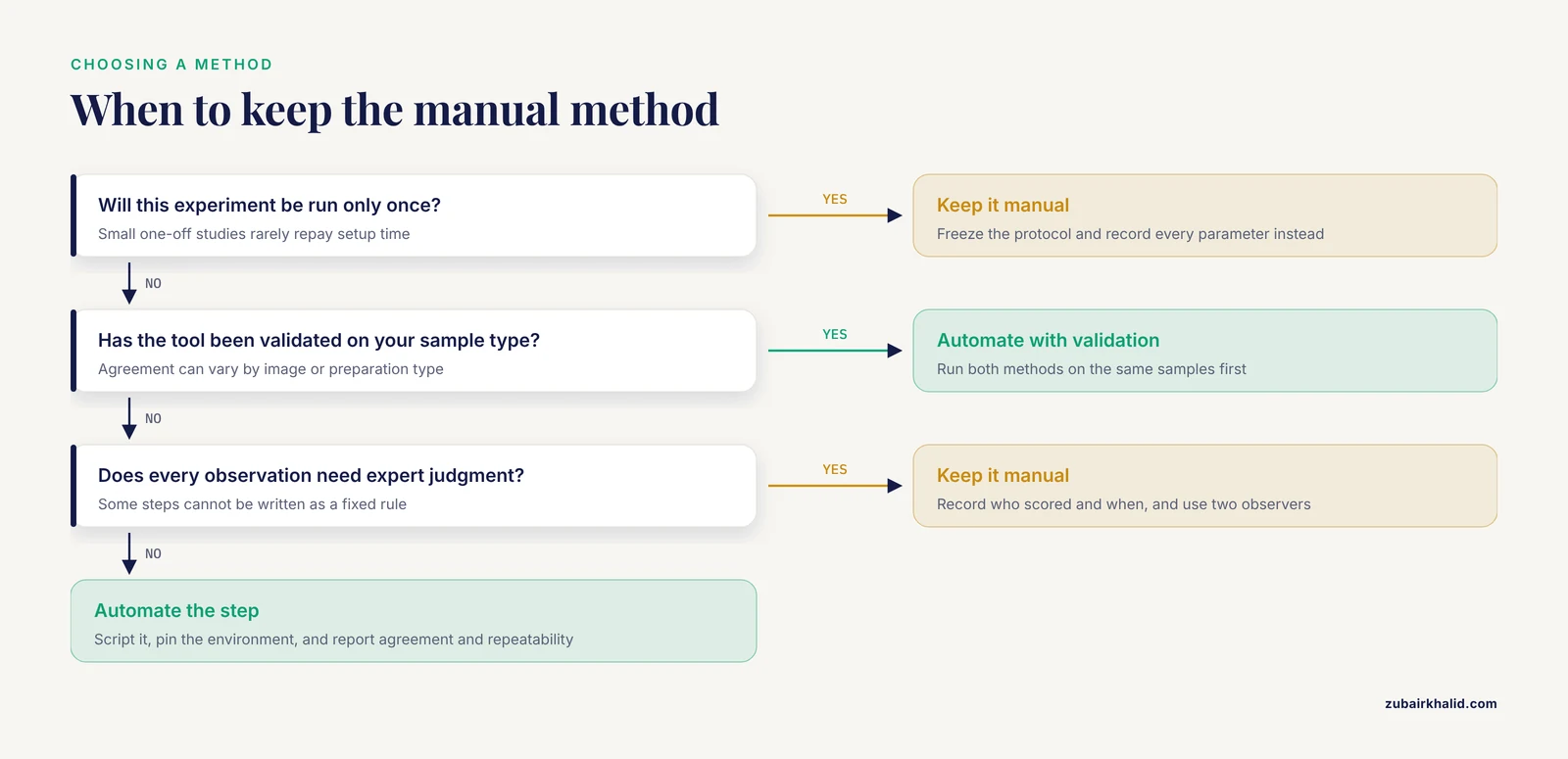
For small experiments run once, for assays where the automated tool has not been validated on your sample type, and for steps requiring genuine expert judgment at every observation. Manual work with a frozen protocol and recorded parameters is still reproducible research.
Sources
- Automation of high-throughput mRNA-seq library preparation: a robust, hands-free and time efficient methodology.
- Pulldown Assay Coupled with Co-Expression in Bacteria Cells as a Time-Efficient Tool for Testing Challenging Protein-Protein Interactions.
- An Atherosclerosis Model in Mice Induced by Both Partial Carotid Ligation and Overexpression of PCSK9.
- A standardized imaging and analysis workflow for quantitative evaluation of cutaneous neurofibromas in Nf1-KO mice.
- A high-throughput and time-efficient Nanopore full-length 16S rRNA gene sequencing protocol for synthetic microbial communities.
- Validation of an Optimized DuraClone Phenotyping Kit Workflow for TBNK Subset Quantification.
- A Simple Migration/Invasion Workflow Using an Automated Live-cell Imager.
- systemPipeR: NGS workflow and report generation environment.
- Dual UHPLC-HRMS Metabolomics and Lipidomics and Automated Data Processing Workflow for Comprehensive High-Throughput Gut Phenotyping.
- Esmraldi: efficient methods for the fusion of mass spectrometry and magnetic resonance images.
- Reproducible Semi-Automated Quantification of Vascularization in Bone Sections Using CD31 Immunohistochemistry and Trainable Weka Segmentation.
- Validation of an automated AI-based micro-CT organ segmentation workflow against expert annotations and its impact on fluorescence quantification.
- Real-Time Global Longitudinal Strain During Echocardiography: A Deep Learning Platform for Improved Workflow.
- Diagonal DWI: A Time-Efficient Alternative to 3-Scan Trace DWI for Breast Lesion Evaluation at 3.0-T MRI-A Phantom Study and Clinical Assessment.
- Deep learning reconstruction enhances bone visualization in zero echo time MRI for cervical spondylosis: A prospective study.
- Purple: A Computational Workflow for Strategic Selection of Peptides for Viral Diagnostics Using MS-Based Targeted Proteomics.
- First Implementation of an All-in-One Solution With Fully Automatic Workflow for Rectal Cancer Based on an Integrated CT-linac.
- Workflow evaluation of a commercial deep learning-based image analysis tool for the quantification of angiogenesis in vivo.