How to Write a Reproducible Analysis Script: Step-by-Step Guide

By Dr. Zubair Khalid, DVM, MS, PhD · 2026-11-11

By the end of this guide you will be able to turn a loose collection of analyses into one reproducible analysis script that runs from raw data to final figures on any computer, record the exact software versions it needs, and package the whole project so a collaborator or reviewer gets identical results. You will need R (version 4.2 or later) or Python (version 3.10 or later), the version control tool git, and optionally Docker. Everything else installs in a few minutes.

A reproducible analysis script is a plain-text file that takes raw data as its only input and produces every number, table, and figure in your report with no manual steps in between. The payoff is concrete. Recent work in metabolomics argues that the practices that make research data findable, accessible, interoperable, and reusable (the FAIR principles) should extend to the analyses themselves, so that raw files, processing choices, and results travel together as one auditable package [1]. The alternative is well documented. Because bioinformatics tools depend on other tools, each with its own release cycle, identical code can produce different results depending on which software versions happen to be installed [2].

What Makes a Script Reproducible

Reproducible research means an independent person can obtain your reported results using your deposited data, code, and a description of the computing environment. Three ingredients make that possible.

Deterministic code. The same input always produces the same output. Random processes are controlled with a fixed seed.
A pinned environment. Every package version, and ideally the operating system layer, is recorded and reinstallable. Frameworks such as FairFlow generate ready-to-run interfaces that execute analyses inside version-locked containers precisely because undocumented dependencies undermine reproducibility [2].
A single execution path. One command runs the entire analysis. Configuration-driven workflows such as scFlowReport propagate one user-defined comparison across multiple downstream analyses and compile the results into a self-contained HTML report that can be shared without a server [3].

A script that only runs on your laptop, with your specific package versions, and only if you click through three dialog boxes in the right order, is not reproducible no matter how clean the code looks.

Install and Prepare Your Tools

Set up the following before writing any analysis code.

R 4.2 or later from CRAN, or Python 3.10 or later from python.org or Miniconda.
RStudio Desktop or Positron (for R users), or VS Code (for Python users).
git, installed from git-scm.com, so every change to the script is tracked.
renv (R) or conda/venv (Python) for pinning package versions.
Docker Desktop, optional but strongly recommended, so your environment can be shipped as an image.

If you prefer not to install anything manually, tools built on top of these foundations can prepare the setup for you. The methylEZ application, for example, generates validated samplesheets and ready-to-run commands for containerized sequencing workflows while preserving transparent, script-first execution [4].

Step-by-Step: Building a Reproducible Analysis Script

Step 1: Set Up a Fixed Project Folder

Create one directory per project, with data kept separate from code and outputs.

mkdir -p myproject/data/raw myproject/data/processed \
         myproject/scripts myproject/results myproject/figures
cd myproject
git init

The rule that matters here is that everything under data/raw/ is immutable. You never edit, rename, or overwrite raw files. Every transformation that produces a file in data/processed/ happens inside the script, so the full chain from raw to result is rerunnable.

Step 2: Pin Your Software Environment

In R, initialize renv inside the project:

install.packages("renv")
renv::init()
renv::snapshot()

renv::snapshot() writes a file called renv.lock that records the exact version of every package your project uses. A collaborator recreates the environment with renv::restore(). In Python, export the environment explicitly:

conda create -n myanalysis python=3.11
conda activate myanalysis
conda env export > environment.yml

A collaborator recreates it with conda env create -f environment.yml. As a lightweight fallback, pip freeze > requirements.txt records Python package versions.

This step is where most irreproducibility is created or prevented. The Julia identifiability tutorial cited throughout this guide's source literature makes every reported result reproducible through companion scripts executed in a pinned and tested Julia environment [5], and the quantitative proteomics pipeline in Methods in Molecular Biology ships complete, version-controlled R scripts with its repository for the same reason [6].

Add a session record at the end of your script so every output carries its own provenance:

sessionInfo()

sessionInfo() prints the R version, operating system, and every loaded package with its version. Write it to a file (capture.output(sessionInfo(), file = "results/sessionInfo.txt")) rather than only to the console.

Step 3: Control Randomness With a Seed

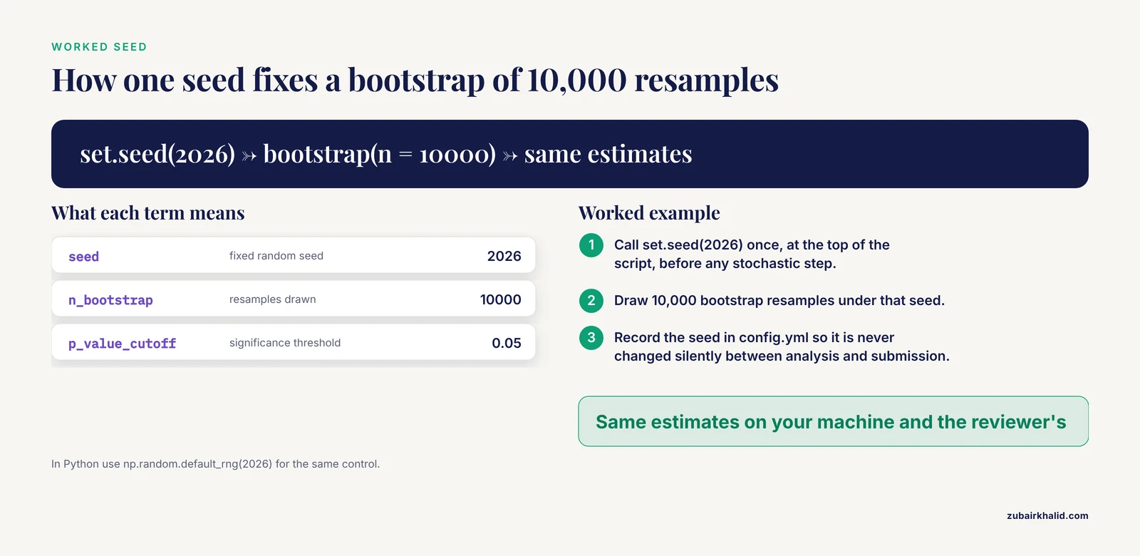
Calculation showing set.seed(2026) feeding a bootstrap of 10,000 resamples so the same estimates appear on the author's and the reviewer's machine.

Any step that involves simulation, resampling, bootstrapping, or random train-test splits must run under a fixed seed.

set.seed(2026)

In Python:

import numpy as np
rng = np.random.default_rng(2026)

set.seed(2026) forces R's random number generator to follow the same sequence of draws every time, so a bootstrap of 10,000 resamples gives the same estimates on your machine and on a reviewer's machine. Pick one seed, record it at the top of the script, and never change it silently between the analysis and the submitted version.

Step 4: Keep Parameters Out of the Code

Hardcoded numbers buried in the middle of a script are the most common source of silent divergence between what a paper says was done and what the code actually does. Move parameters into a configuration file.

Create config.yml:

p_value_cutoff: 0.05
min_fold_change: 1.5
n_bootstrap: 10000
seed: 2026
input_file: "data/raw/counts.csv"
output_dir: "results"

Read it once at the top of the script. Configuration-driven design is the organizing principle behind tools such as scFlowReport, where a single user-defined comparison drives the whole downstream analysis [3], and the spatial transcriptomics protocol by Wang and colleagues recommends documenting an explicit rationale for each parameter choice alongside the script itself [7]. When thresholds like a p-value cutoff or a minimum fold change live in the config file, updating the analysis for revision two means changing one line, not hunting through two hundred lines of code.

Step 5: Read Raw Data Read-Only and Write Derived Files

Your script should open raw files, never save back to them, and write every intermediate and final product to a new location.

raw <- read.csv("data/raw/counts.csv")
clean <- raw[complete.cases(raw), ]
write.csv(clean, "data/processed/counts_clean.csv", row.names = FALSE)

This gives you an auditable chain. If a collaborator questions a result, you can inspect counts_clean.csv without touching the original data. Pipelines that process mass spectrometry data formalize the same idea by emitting a fully populated document for every analytical plate so that results can be reimported and rechecked [8].

Step 6: Structure the Analysis in Ordered Sections

Write the script top to bottom in numbered, commented sections: load libraries, load config, load data, clean, model, plot, save. R users should consider literate formats such as R Markdown or Quarto, which interleave code and prose. The Metabonaut educational resource teaches this approach explicitly, pairing executable workflows with prose explanations so readers learn the reasoning, not just the commands [1]. A well-annotated example in the same style is the cost-effectiveness meta-analysis tutorial in Pharmacoeconomics, which provides fully annotated R scripts so each harmonization and pooling step can be read and rerun [9].

A minimal section header pattern:

## 1. Libraries ----
## 2. Configuration ----
## 3. Data import ----
## 4. Quality control ----
## 5. Statistical model ----
## 6. Figures ----
## 7. Session record ----

Step 7: Save Outputs With Traceable Names

Every figure and table gets an explicit filename derived from its parameters, not a vague default like plot.png or Rplot01.pdf.

ggsave(file.path("figures",
      paste0("volcano_fc", cfg$min_fold_change,
             "_p", cfg$p_value_cutoff, ".pdf")),
      volcano_plot, width = 6, height = 5)

A reviewer who sees volcano_fc1.5_p0.05.pdf knows exactly which settings produced it. Workflows such as scFlowReport go further and automatically compile figures and summary tables into a standardized, self-contained report, which removes the manual harmonization of heterogeneous outputs that otherwise invites errors [3].

Step 8: Run the Whole Script From a Clean Start

Restart R (Session, Restart R in RStudio) or open a fresh shell, then execute the script end to end:

Rscript scripts/analysis.R

or, for a literate document:

rmarkdown::render("analysis.Rmd")

If the script only works when you run it in pieces, in a particular order, with objects left over from yesterday's session, it is not yet reproducible. The clean-start test is the single fastest way to find missing library calls, unrecorded intermediate steps, and files that are read from the wrong folder. Protocols designed for teaching, including the spatial transcriptomics workflow in the Journal of Visual Experiments, build in explicit troubleshooting checkpoints for exactly this reason [7].

Step 9: Package the Environment in a Container

For full portability, put the pinned environment inside a Docker image. A minimal Dockerfile for an R project:

FROM rocker/r-ver:4.4.1
RUN Rscript -e 'install.packages(c("dplyr","ggplot2"))'
COPY scripts/ scripts/
COPY config.yml config.yml
CMD ["Rscript", "scripts/analysis.R"]

Build and run:

docker build -t myanalysis .
docker run --volumes-from data -it myanalysis

FROM rocker/r-ver:4.4.1 fixes the R version and the underlying operating system libraries. Anyone with Docker gets byte-for-byte comparable behavior regardless of their own installation. This is the approach taken by containerized mass spectrometry workflows, which pin third-party tools in version-controlled Docker images with Apptainer support for high-performance computing clusters [8], and by FairFlow, which automatically generates language-specific interfaces that each execute the analysis inside a version-locked container [2].

Step 10: Version Control and Share

Commit every change:

git add scripts/analysis.R config.yml renv.lock
git commit -m "Add QC filtering and session record"
git push

When you share the repository, include the lock file, the raw or simulated data (or a download script), the config file, and a README with the one-line run command. Repositories built around reproducible analysis follow this pattern deliberately. The ECOTEC student risk dataset release pairs its data with variable-level metadata, validation scripts, benchmark scripts and outputs, software-environment specifications, and FAIR-oriented documentation [10]. Metabonaut makes the same point from the teaching side: the goal is to carry FAIR practice from the data all the way through the analysis [1].

Worked Example: A Minimal Reproducible Script

Here is a complete, self-contained R script that follows every step above.

## 1. Libraries ----
library(ggplot2)

## 2. Configuration ----
cfg <- list(
  seed = 2026,
  n_per_group = 50,
  p_cutoff = 0.05
)

## 3. Data ----
set.seed(cfg$seed)
df <- data.frame(
  group = rep(c("control", "treated"), each = cfg$n_per_group),
  value = c(rnorm(cfg$n_per_group, mean = 10, sd = 2),
            rnorm(cfg$n_per_group, mean = 11.2, sd = 2))
)

## 4. Model ----
fit <- t.test(value ~ group, data = df)

## 5. Figure ----
p <- ggplot(df, aes(group, value)) +
  geom_boxplot() +
  theme_minimal()
ggsave("figures/group_comparison.pdf", p, width = 5, height = 4)

## 6. Save results ----
dir.create("results", showWarnings = FALSE)
writeLines(
  c(paste("p_value:", signif(fit$p.value, 3)),
    paste("mean_difference:", signif(diff(fit$estimate), 3))),
  "results/t_test_summary.txt"
)

## 7. Session record ----
capture.output(sessionInfo(), file = "results/sessionInfo.txt")

Run with Rscript scripts/analysis.R. Expected behavior: the script creates figures/group_comparison.pdf, writes results/t_test_summary.txt containing the p-value and the mean difference between groups, and writes results/sessionInfo.txt. Because the seed is fixed at 2026, the simulated data, the test statistic, and the figure are identical on every machine running the same R version recorded in sessionInfo.txt. If you delete the results/ and figures/ folders and rerun, you get the same files back. That delete-and-rerun test is your basic quality check.

To verify the result is right, ask three questions. Does the script run from a fresh R session with no errors? Do the saved numbers match what you report? Does the session record show the package versions you intended?

Reproducibility Checklist

Use this reproducibility checklist before you submit or share any analysis.

Raw data are read-only and stored separately from derived data.
One command runs the entire analysis from a clean session.
A random seed is set before any stochastic step.
All thresholds and parameters live in a config file or at the top of the script.
Package versions are pinned (renv.lock, environment.yml, or requirements.txt).
sessionInfo() or an equivalent record is saved with the outputs.
Every figure and table filename encodes its parameters.
The script contains no setwd(), absolute paths, or manual GUI steps.
The environment is packaged in a Docker image (or equivalent container).
The repository includes the lock file, config, data or data-download script, and README.
A collaborator has run it successfully on a different machine.
The analysis is described in prose alongside the code, in a literate document or well-commented script.

Items 1 through 6 prevent most failures. Items 9 through 12 separate a script that works for you from a script that works for science.

Key Commands at a Glance

Command	What it does	When to run it
`set.seed(2026)`	Fixes the random number stream	Once, before any stochastic step
`renv::init()`	Activates project-local package library	When starting the project
`renv::snapshot()`	Writes renv.lock with exact package versions	After adding or updating packages
`renv::restore()`	Rebuilds the environment from renv.lock	On a new machine or container
`conda env export > environment.yml`	Records the full conda environment	After installing packages
`sessionInfo()`	Prints R version, OS, and package versions	End of every script
`rmarkdown::render("analysis.Rmd")`	Executes the whole document from scratch	Before every share or submission
`docker build -t myanalysis .`	Bakes code and environment into an image	Before releasing or archiving
`git commit -m "message"`	Snapshots the current state of the project	After every meaningful change

Common Mistakes and Limitations

Absolute paths and setwd(). A script that begins with setwd("C:/Users/you/Desktop/final_FINAL_v3") fails on every other computer. Use relative paths anchored at the project root, ideally through an RStudio Project or a working-directory check at the top of the script.

Unrecorded package versions. The single most cited cause of irreproducible computational results is undocumented dependencies, since tool updates for bug fixes and new features can change numerical output [2]. Record versions before you need them, not when a reviewer asks.

Manual steps hiding inside the workflow. Ad hoc point-and-click quality control is a documented source of user- and laboratory-level variation in targeted mass spectrometry, which is why automated pipelines consolidate those steps into scripted, reportable modules [8]. If you adjusted a threshold interactively in ImageJ or Excel, that adjustment does not exist until it is written into the script or config file.

Unstated analytic choices. A recent evaluation of scripts generated from natural-language queries found that when a prompt left a choice unstated, the generated analyses diverged, showing that reproducibility depends on both the code and the explicit decisions behind it [11]. The same applies to human-written scripts. If two reasonable analysts could read your script and legitimately choose different cutoffs, record which one you used and why.

Assuming one pipeline equals another. Different valid tools can give materially different answers on the same data. In a benchmark of organelle quantification pipelines across microscopy platforms, droplet counts and size distributions varied substantially between pipelines and imaging modalities even when segmentation looked qualitatively consistent [12]. Reproducibility means your script gives your reported numbers, not that any pipeline would have found the same biology.

Not testing on a fresh machine. Scripts accumulate invisible dependencies on the author's setup. Hand the repository to a colleague, or spin up a clean container, before you declare it finished.

A limitation to state plainly. A reproducible script guarantees that results can be regenerated, not that the statistical model, the data quality, or the biological interpretation is correct. Reproducibility is a necessary floor for credible analysis, and it works best alongside preregistered design, adequate controls, and independent validation.

Frequently Asked Questions

What exactly is a reproducible analysis script?

A reproducible analysis script is a plain-text file that runs from raw data to final results in one pass, with pinned software versions, a fixed random seed, and no manual steps, so anyone can regenerate your exact outputs.

Do I need to learn the command line to write reproducible scripts?

No. RStudio and graphical tools cover most of the workflow, and applications such as methylEZ now generate ready-to-run commands for beginners while keeping the underlying execution script-first [4]. One shell command, Rscript scripts/analysis.R, is enough to run the finished script.

How is a reproducible script different from a well-commented script?

Comments explain what code does, but reproducibility requires that the code, the data, the parameters, and the exact software environment all travel together and rerun cleanly. A well-commented script without a lock file or seed can still produce different numbers on a different computer.

What is the quickest reproducibility check on my own machine?

Restart R or open a fresh terminal, delete your results and figures folders, and run the entire script with a single command. If any step fails or any output changes, you have found an irreproducibility you can fix immediately.

Do I always need Docker?

No. A pinned environment with renv or conda covers most projects. Docker earns its cost when your analysis depends on system libraries, multiple languages, or tools that colleagues on different operating systems will struggle to install [2].

How do I handle very large data files that should not go in a git repository?

Keep the repository for code, config, and lock files, and store raw data in an institutional or public archive such as MetaboLights or a data repository. Include a small download or import script so the pipeline can fetch the data itself, following the FAIR-oriented repository pattern used by shared dataset releases [10].

Can AI assistants write reproducible scripts for me?

They can draft code, but reproducibility depends on stated choices, not just generated code. An evaluation of AI-generated epidemiology scripts found that outputs diverged whenever a prompt left an analytic choice unstated, even though the generated code stayed within the declared data dictionary [11]. Treat the assistant as a first-draft writer and you as the person who pins every decision.

What should I put in my README for a reproducible analysis?

Four things: the one-line command that runs the analysis, instructions for recreating the environment from the lock file, a description of the expected folder structure and outputs, and the point of contact for questions. Reviewers and collaborators should be able to go from clone to result without emailing you.