How to Create Your First R Markdown Report: A Step-by-Step Tutorial
By Dr. Zubair Khalid, DVM, MS, PhD ·

By the end of this tutorial you will be able to create an R Markdown file, write a YAML header, insert and run code chunks, knit the file into a polished HTML report, and apply a reproducibility checklist so that a colleague can rerun your analysis from scratch and get the same numbers. You need R installed on your computer, and RStudio is strongly recommended because it gives you buttons for everything described here. Total setup time on a standard laptop is under 30 minutes if you already have R, and about an hour if you are starting from zero.
This walkthrough assumes no prior experience with R Markdown. Every command appears in a code block, and every block shows what the expected output looks like on your screen.
Why R Markdown Matters for Reproducible Research
Reproducible research means that another person, or you yourself six months later, can take your data and your analysis code and arrive at the same results, figures, and tables that appear in your report. In fields such as metabolomics, the analysis steps that turn raw instrument files into published feature tables have historically been difficult to share, audit, and reuse, which is exactly the gap that script-based workflows and literate programming aim to close [1]. In applied health research, tutorials now routinely demonstrate full multi-step statistical protocols written entirely in the R environment, so that psychometric analyses can be integrated into substantive studies rather than farmed out to proprietary software [2].
R Markdown supports this goal through literate programming, a term coined by Donald Knuth. The idea is that your document mixes three elements in one file: narrative text that explains what you did, executable R code that does it, and the outputs that the code produces. When you knit the file, R executes every chunk in order from a fresh session and weaves the results into the final document. Nothing you paste manually into a Word file can drift out of sync with the analysis, because the numbers in the report come directly from the code that produced them.
The alternative, copying results from an R console into a word processor, breaks easily. Change one filter in your analysis and every p-value, figure, and table in the manuscript needs manual updating. R Markdown makes the update a single click.
Step 1: Install R, RStudio, and the Required Packages
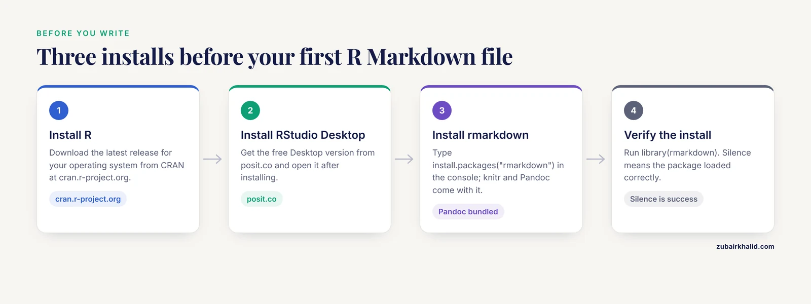
R Markdown depends on three layers, and each layer needs its own install.
Install R. Download the latest release for your operating system from CRAN, the Comprehensive R Archive Network, at cran.r-project.org. On Windows, run the installer and accept the defaults. On macOS, pick the correct installer for your chip type, which the CRAN page labels clearly.
Install RStudio Desktop. RStudio, now called Posit RStudio, is the graphical interface that most R users work in. Download the free Desktop version from posit.co. Open it after installing. You should see three panels: the console on the left, and environment, history, files, and plots panels on the right.
Install the rmarkdown package. Open the RStudio console and type:
install.packages("rmarkdown")R will download rmarkdown and its dependencies, including the knitr package that actually runs your code chunks. This step also installs Pandoc, a document converter that RStudio bundles, so you do not need to install Pandoc yourself.
Verify the install by running:
library(rmarkdown)If nothing happens, that is success. In R, silence after a library call means the package loaded. If you see an error such as there is no package called 'rmarkdown', return to the install.packages() step and check your internet connection.
Step 2: Create Your First R Markdown File
In RStudio, go to the menu and choose File, then New File, then R Markdown. A dialog appears. Leave the Document option selected, enter a title such as My First Reproducible Report, and enter your name in the Author field. Choose HTML as the default output format, which is the most forgiving format for a first attempt because it renders in any web browser with no extra software.
Click OK. RStudio creates a new file with a .Rmd extension containing a short template. Close the template's example content for now. Your file should start with something like this:
---
title: "My First Reproducible Report"
author: "Your Name"
date: "2026-11-11"
output: html_document
---
Save the file immediately with File, then Save As, and give it a descriptive name such as first-report.Rmd. Save it in a new, empty folder dedicated to this project. Folder discipline matters more than most beginners expect, and the section on workflow below explains why.
Step 3: Understand the YAML Header
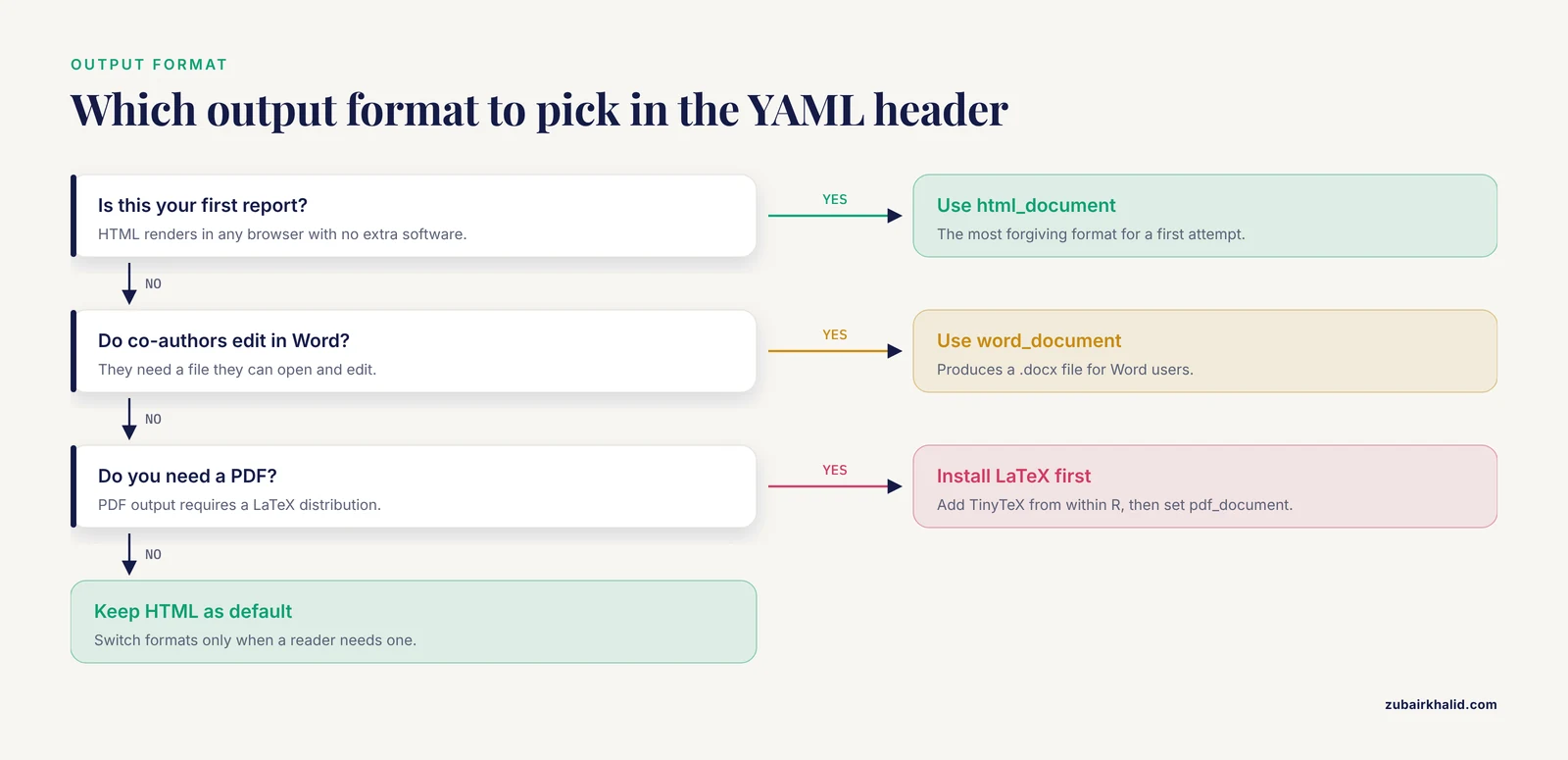
YAML (which stands for YAML Ain't Markup Language, a recursive joke in the naming) is the block of metadata between the two triple-dash lines at the top of your file. Everything there controls how the final document looks and behaves.
The most important field for a first report is output. The value html_document produces a web page. Change it to word_document to produce a .docx file for co-authors who edit in Word, or pdf_document to produce a PDF. PDF output requires a LaTeX distribution, and installing one is an extra step, so keep HTML as your default while learning.
Useful header options for an HTML report include:
---
title: "My First Reproducible Report"
author: "Your Name"
date: "2026-11-11"
output:
  html_document:
    toc: true
    toc_depth: 2
    number_sections: true
    code_folding: hide
---
Each sub-option indents two spaces under html_document. YAML is strict about indentation, and a single extra space produces a parse error. The options shown here add a clickable table of contents (toc), number your headings (number_sections), and add buttons that let readers hide or show your code (code_folding), which is useful when you send the report to a supervisor who cares about results rather than code.
Step 4: Write Text and Code Chunks
An R Markdown file has two kinds of content. Regular text is written in Markdown, a lightweight formatting syntax. R code lives in fenced blocks called chunks, which start with three backticks, a lowercase r inside curly braces, and end with three backticks.
Type this into your file below the YAML header:
This report analyzes a small dataset of plant heights.
knitr::opts_chunk$set(echo = TRUE)
heights <- c(12.4, 13.1, 11.8, 14.2, 12.9, 13.5) mean(heights)
Then click the green arrow at the top right of the chunk, or press Ctrl+Shift+Enter (Cmd+Shift+Enter on a Mac). The chunk runs and the output appears directly beneath it in your editor:
[2] 12.98333That `` is simply R's label for the first value in the result line. You have now executed your first chunk inside a literate document.
Chunk Options That Actually Matter
Every chunk accepts options in its header line. These control what appears in the knitted report and how the code behaves. The setup chunk, named setup with include=FALSE, sets defaults for the whole document.
| Option | What it does | When to use it |
|---|---|---|
echo | Shows or hides the code in the output | echo=FALSE for a report aimed at non-programmers |
eval | Runs or skips the code | eval=FALSE to show code you do not want executed |
include | Runs the code but hides both code and output | Setup and package-loading chunks |
message | Shows or hides package startup messages | message=FALSE to keep the report clean |
warning | Shows or hides R warnings | warning=FALSE for final reports, keep on while debugging |
cache | Stores chunk results and reuses them | cache=TRUE for slow steps such as large model fits |
fig.width, fig.height | Sets plot size in inches | fig.width=6, fig.height=4 for standard figures |
A common pattern for a data-analysis report is a hidden setup chunk with echo = FALSE, message = FALSE, warning = FALSE as global defaults, followed by visible chunks for the analysis steps you want readers to see.
Inline Code
Text can also pull numbers directly from R. Write a single backtick, the letter r, your code, and a closing backtick, all on one line of prose:
The mean plant height was `r round(mean(heights), 1)` cm.When knitted, this sentence prints as: The mean plant height was 13.0 cm. If the data change, the sentence updates itself. This single feature eliminates the most common source of discrepancy between analysis scripts and manuscripts.
Step 5: Knit Your First Report
Click the Knit button at the top of the editor pane, or press Ctrl+Shift+K. RStudio starts a fresh R session, runs every chunk in order from the top of the file, and opens the finished HTML document in a viewer window.
Watching the R Markdown console while it knits tells you what is happening. A successful knit ends with a line like this:
Output created: first-report.htmlThe HTML file appears in the same folder as your .Rmd file. Open it in a browser to confirm it renders correctly.
Reading the Knit Log
While knitting, the console prints each chunk name followed by its running time:
processing file: first-report.Rmd
 |setup          |  0 ms |
 |load-data      | 40 ms |
This log is your friend. A chunk that takes 40 seconds to knit every time is a candidate for cache=TRUE. The log also shows exactly which chunk failed if something goes wrong, with the file line number in the error message.
Step 6: Add Plots, Tables, and a Complete Mini-Analysis
A report with one mean is not yet a report. Extend your file with a plot and a table. Type this new chunk:
plot(heights, pch = 19, col = "darkgreen", xlab = "Plant number", ylab = "Height (cm)", main = "Plant heights in trial 1") abline(h = mean(heights), lty = 2)
Knit again. A scatterplot of the six heights appears in the report, with a dashed horizontal line marking the mean. Because the figure is produced by code, changing the data and re-knitting regenerates the figure automatically.
For tables, the knitr::kable() function converts a data frame into a formatted table:
heights_df <- data.frame(height_cm = heights) knitr::kable(summary(heights_df), digits = 1, caption = "Summary of plant heights")
This pattern scales directly to real analyses. Published tutorials demonstrate exactly this structure for complex protocols, such as a six-step psychometric workflow in R that moves from item distributions through factor analysis to reliability and global scores, all documented in a single reproducible script [2]. Your plant-height example is structurally identical, just smaller.
Step 7: Build a Reproducible Workflow Around the File
A knittable file is necessary but not sufficient for reproducible research. Modern guidance, including the FAIR principles extended from data to research software and workflows, emphasizes that the whole analysis environment should be shareable and auditable, not just the code [1]. Three habits get you most of the way there.
Record your session information. Add this chunk at the very end of every report:
sessionInfo()
The output lists your R version, operating system, and the exact version of every attached package. A colleague reading your report can immediately see whether a version difference might explain a result that does not match theirs.
Set a random seed whenever randomness is involved. Functions that bootstrap, permute, or split data sample randomly. Without a seed, results differ on every run. Fix it once at the top of your analysis:
set.seed(42)Place this before any code that uses random sampling, and document which seed you used.
Use relative paths. Never write read.csv("C:/Users/you/Desktop/project/data.csv"). That path only exists on your computer. Instead, keep the data file in your project folder and load it with a path relative to the report:
heights <- read.csv("data/heights.csv")For robust path handling across operating systems, the here package finds your project root automatically:
install.packages("here")
here::here("data", "heights.csv")
Consider renv for package versions. The renv package records the exact package versions your project used in a lockfile, so a collaborator can restore that same environment. It goes beyond what a one-line tutorial can cover, but knowing it exists tells you where to look once basic reports feel routine.
A Reproducibility Checklist
Before you send any R Markdown report to a supervisor, reviewer, or collaborator, run through this list:
- The file knits from a fresh session with no errors, verified by restarting R (Session menu, then Restart R and Run All Chunks) before the final knit.
set.seed()appears before any stochastic analysis.sessionInfo()output is included at the end of the document.- All file paths are relative or built with
here::here(). - No results are hard-coded into prose, figures, or tables. Every number comes from inline code or a chunk.
- The data files live in the project folder, or the code downloads them from a stable archive.
- Package installation happens in a documented script or the environment is locked with renv.
- Chunk options hide distracting messages but keep the analytical code visible.
Common Mistakes and Limitations
Object not found. The most frequent beginner error. Its message looks like:
Error in mean(heights) : object 'heights' not foundIt happens when a chunk uses an object that a previous chunk never created, typically because you ran chunks out of order interactively or renamed a variable. The fix is to knit from a clean session, since knitting always runs everything in order from the top. If the knit itself fails with this error, some chunk earlier in the file failed or was skipped.
YAML parse error. A message such as Parser error: while parsing a block mapping almost always means an indentation problem in the header. Sub-options under output: must be indented exactly two spaces, and strings containing colons must be wrapped in quotation marks.
could not find function. This error means a package is not loaded:
Error in knitr::kable(...) : could not find function "knitr::kable"Add library(knitr) in your setup chunk, or check the spelling of the package name. Names are case sensitive.
The knit produces a stale result. Caching is convenient and dangerous. If you change the code inside a cached chunk, knitr usually detects it and reruns, but changes to a function used by that chunk, or to an external data file, can go unnoticed. Clear the cache with the broom icon in the RStudio chunk toolbar, or delete the _cache folder, whenever results look suspicious.
Editing the HTML file instead of the Rmd. The HTML, Word, or PDF output is disposable. Never edit it directly. All changes go into the .Rmd file, and you regenerate the output by knitting. Losing track of this is the classic way to lose work.
Pasting results into the text. Hard-coding a p-value into a sentence defeats the purpose of literate programming. Use inline code references so the text and the analysis stay synchronized.
Limitations of the approach itself. R Markdown solves reproducibility of the analysis, not reproducibility of the entire scientific context. It cannot record instrument calibration, sample collection conditions, or lab notebook details. For workflows that begin with raw instrument files, published educational resources combine R Markdown-style literate documents with version control and public data deposition to carry FAIR practice from the data all the way through the analysis [1]. Also, a document that knits on your machine today is not guaranteed to knit in five years, because packages change. Session information and lockfiles are the partial remedy. Individual research projects with unusual requirements, such as compliance with specific journal data policies, need project-specific planning beyond what any general template provides.
Frequently Asked Questions
Do I need to be an expert in R before writing an R Markdown report?
No. If you can run a function like mean() and plot(), you can write a useful R Markdown report, and your R skills and reporting skills will improve together.
What is the difference between R Markdown and Quarto?
Quarto is the newer publishing system from the same team that builds R Markdown, and it works with R, Python, and Julia. R Markdown remains fully supported and everything in this tutorial applies to it.
Can I use R Markdown with Python or other languages?
Yes. R Markdown chunks can run Python, SQL, Bash, and several other engines by specifying the language in the chunk header, such as {python}.
Why does my report look different when my colleague knits the same file?
Different package versions, different operating systems, or a missing set.seed() can all change output. Include sessionInfo() output and fix your seed to narrow down the cause.
How do I convert my R Markdown report to PDF?
Change the YAML output to pdf_document and knit. You must first install a LaTeX distribution, such as TinyTeX, which you can add from within R with the tinytex package.
Is R Markdown still worth learning if Quarto is newer?
Yes. An enormous amount of existing documentation, course material, and published workflows use R Markdown, and the skills transfer directly to Quarto.
How do I stop my report from showing all the warning messages?
Set warning=FALSE and message=FALSE in your setup chunk. Do this only in a final report, because while you are still analyzing data, warnings often reveal real problems.
Where can I find real-world examples of full R Markdown workflows?
Published tutorials in the health and life sciences demonstrate complete script-based protocols in R, from data checks through final summary statistics, and open educational resources in metabolomics show executable workflows that take raw data through to annotated results [2] [1].