How to Migrate from SPSS to R
By Dr. Zubair Khalid, DVM, MS, PhD ·

By the end of this guide you will be able to open an SPSS data file in R, preserve your variable and value labels, translate a typical SPSS workflow (descriptives, t-test, regression) into R commands, and verify that your results match what SPSS would have produced. To follow along you need a computer with internet access, your SPSS data saved as a .sav file, and about two hours for the first pass.
Why Researchers Switch from SPSS to R
SPSS has been the default statistics package in many psychology, nursing, education, and social science programs for decades. It handles the standard analyses well and its point-and-click menus are easy to learn. R is a programming language built for statistics, and it competes with SPSS on every analysis SPSS can run while adding capabilities SPSS lacks.
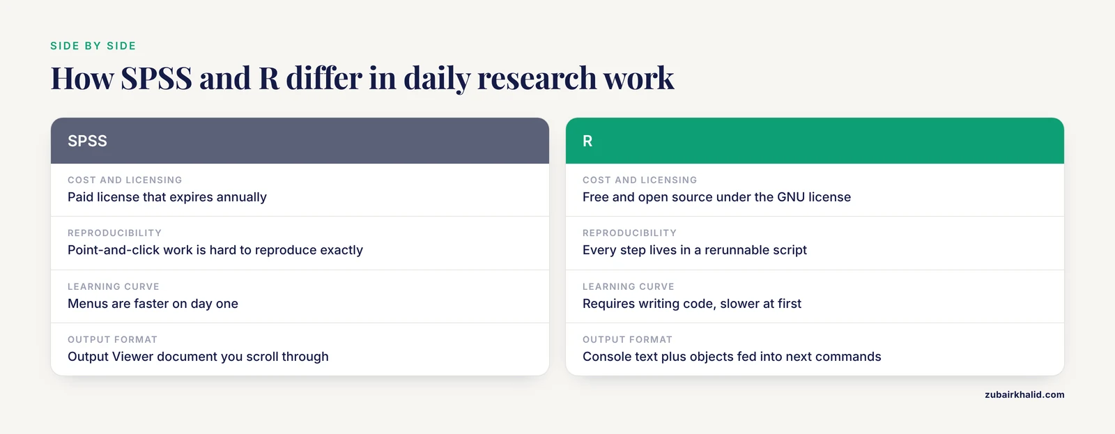
A fair research software comparison comes down to four practical differences:
- Cost and licensing. SPSS requires a paid license that expires annually. R is free and open source under the GNU General Public License, so there is no license to renew and no restriction on how many machines you install it on.
- Reproducibility. SPSS point-and-click work is hard to reproduce exactly. Every step in R lives in a script file, so you (or a reviewer) can rerun the entire analysis from raw data to final table with one command.
- Scale and flexibility. R handles datasets that strain SPSS, and the Comprehensive R Archive Network (CRAN) hosts thousands of add-on packages for specialized methods, from Bayesian models to text mining.
- Learning curve. SPSS menus are faster on day one. R requires writing code, which costs time upfront and pays off for every project after that.
For students and researchers deciding on the best software for their work, the honest answer is that SPSS and R can run the same t-tests, ANOVAs, and regressions. The choice is about workflow, cost, and career direction. Many statistics departments and journals now expect at least basic R skills, and learning R while SPSS is still installed on your machine is a reasonable transition strategy.
What You Need Before You Start
Install these two programs before touching any data:
- R itself. Download the current release for Windows, macOS, or Linux from CRAN at
https://cran.r-project.org. The installer takes a few minutes. - RStudio Desktop (now called Posit). This is the interface most people use to write R code. Download the free Desktop version from
https://posit.co/download/rstudio-desktop/. It requires R to already be installed.
RStudio is not a different language. It is a workspace with four panes: a script editor where you write code, a console where code runs, an environment pane listing your data and variables, and a files and plots pane.
You also need your SPSS data. If your file is .sav, R can read it directly. If your data lives only inside an SPSS session, open SPSS and save it with **File > Save As > SPSS Statistics (.sav)* before you close the program.
Migrating from SPSS to R Step by Step
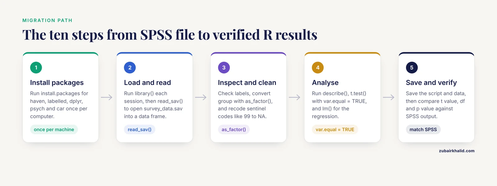
This walkthrough uses a hypothetical dataset called survey_data.sav with an anxiety score, a group variable (1 = control, 2 = treatment), study hours, and an exam score. Every command below runs in the RStudio console or in a script you can save and rerun.
Step 1: Open RStudio and install the packages you need
Packages are add-ons that extend base R. Type this in the console and press Enter:
install.packages(c("haven", "labelled", "dplyr", "psych", "car"))The haven package reads and writes SPSS files. The labelled package works with variable and value labels. dplyr handles data manipulation, psych computes descriptive statistics and reliability, and car provides companion tests such as Levene's test for homogeneity of variance. Installation takes a minute or two per package and you only do it once per computer.
If the console prints a message like:
There is no package called 'haven'when you later try to use it, the package was not installed on that machine. Rerun install.packages("haven").
Step 2: Load the packages for this session
Installing a package makes it available. Loading it makes it active:
library(haven)
library(dplyr)
You must run library() at the start of every R session. A common beginner habit is to put all library() calls at the top of the script so rerunning the script from a clean state works.
Step 3: Read the SPSS file into R
Set your working directory to the folder containing your data, or give the full path:
survey <- read_sav("survey_data.sav")The read_sav() function takes one required argument, the file path, and returns a data frame, which is R's version of a rectangular dataset with rows and columns. The <- symbol assigns the result to an object named survey. In SPSS the file opens into a visible spreadsheet window. In R the data loads silently into memory. Nothing prints, and that silence means success.
If the file path is wrong you will see:
Error: 'survey_data.sav' does not exist in current working directoryFix this by checking the file name and location, or by running getwd() to see which folder R is looking in and setwd() to change it.
Step 4: Inspect the data and its labels
SPSS stores two things R preserves on import: variable labels (long descriptions such as "State anxiety score at baseline") and value labels (the mapping of 1 = "Control", 2 = "Treatment"). View them:
dplyr::glimpse(survey)
labelled::var_label(survey)
labelled::val_labels(survey$group)
Expected output for the value labels looks like this:
   1        2
Control Treatment
Numbers stored in SPSS with value labels arrive in R as haven_labelled numerics. They print as numbers (1, 2) rather than words, which confuses many new users. To make the labels active in analysis and plotting, convert key variables to factors, which are R's categorical variables:
survey$group <- as_factor(survey$group)The as_factor() function replaces the numeric codes with their labeled text values while keeping the underlying ordering.
Step 5: Handle missing values the SPSS way
In SPSS you often declare user-defined missing values, for example coding "refused to answer" as 99. When haven imports the file, those codes become tagged missing values (special NA values that remember their original code). If your SPSS file never declared user-missing values, codes like 99 arrive as ordinary numbers and will silently corrupt your means and correlations.
Check for this and fix it explicitly:
summary(survey$income)
survey$income[survey$income == 99] <- NA
After this replacement, any function that computes a statistic will exclude the NA values, mirroring SPSS listwise or pairwise exclusion depending on the function. This single check prevents the most damaging silent error in the whole migration.
Step 6: Compute descriptive statistics
The SPSS DESCRIPTIVES procedure maps to summary() for a quick view or psych::describe() for a table resembling SPSS output:
summary(survey$anxiety)
psych::describe(survey[, c("anxiety", "study_hours", "exam_score")])
Expected output from describe() includes columns for mean, sd, median, min, max, skew, and se, one row per variable:
             vars  n  mean    sd median trimmed   mad min max range skew
anxiety         1 100 42.35  9.87   42.00   42.10 10.38  20  70    50 0.21
study_hours     2 100  6.42  3.11    6.00    6.31  2.97   0  15    15 0.34
exam_score      3 100 71.80 12.44  72.50   71.95 12.60  38  98    60 -0.15
The frequencies procedure maps to table():
table(survey$group) Control Treatment
48 52 Step 7: Run an independent-samples t-test
Here is where small differences between the programs matter. SPSS's independent-samples t-test output shows both equal-variances and unequal-variances rows. R's t.test() defaults to the unequal-variances version (Welch's t-test). To reproduce the SPSS "equal variances assumed" row, set var.equal = TRUE:
t.test(anxiety ~ group, data = survey, var.equal = TRUE)The ~ symbol reads as "predicted by" and means compare anxiety across the two levels of group. Expected output:
	Two Sample t-test

data:  anxiety by group
t = -2.1859, df = 98, p-value = 0.03118
alternative hypothesis: true difference in means between group Control and group Treatment is not equal to 0
95 percent confidence interval:
 -6.3825111 -0.3136427
sample estimates:
   mean in group Control mean in group Treatment
                 44.21583                 41.41765
Most parameters of t.test() have SPSS equivalents. The paired = TRUE argument runs a paired-samples test, alternative = "less" or "greater" runs one-tailed tests, and conf.level = 0.99 changes the confidence interval from the default of 0.95. Before comparing results, check the homogeneity of variance assumption the same way you would in SPSS:
car::leveneTest(anxiety ~ group, data = survey)Step 8: Run a linear regression
SPSS REGRESSION maps directly to lm(), which stands for linear model:
model <- lm(exam_score ~ study_hours + anxiety, data = survey)
summary(model)
Expected output:
Call:
lm(formula = exam_score ~ study_hours + anxiety, data = survey)

Residuals:
    Min      1Q  Median      3Q     Max
-25.511  -7.893   0.314   7.622  24.708

Coefficients:
            Estimate Std. Error t value Pr(>|t|)
(Intercept)  52.3104     4.8821  10.714  < 2e-16 ***
study_hours   2.4512     0.3817   6.421 8.7e-09 ***
anxiety      -0.3207     0.1202  -2.668  0.00897 **
---
Signif. codes:  0 '***' 0.001 '**' 0.01 '*' 0.05 '.' 0.1 ' ' 1

Residual standard error: 11.42 on 97 degrees of freedom
Multiple R-squared:  0.3512,	Adjusted R-squared:  0.3379
F-statistic: 26.26 on 2 and 97 DF,  p-value: 5.6e-10
Each coefficient row matches the SPSS regression table: unstandardized B (Estimate), standard error, t value, and p value. R prints standardized betas separately if you scale your variables first with scale(). To get a clean table of coefficients for a manuscript, the broom package converts model output into a tidy data frame.
Step 9: Save your work
Save the cleaned data in two formats:
saveRDS(survey, "survey_clean.rds")
haven::write_sav(survey, "survey_clean.sav")
saveRDS() is R's fast native format and preserves all labels and factor structure exactly. write_sav() writes a real SPSS file so a colleague still using SPSS can open your cleaned dataset. For the analysis itself, save the script file (in RStudio, File > Save), because the script is the equivalent of your SPSS syntax plus your point-and-click history combined.
Step 10: Verify that R and SPSS agree
Before trusting R for a real project, run one analysis you have already done in SPSS and compare the numbers. If you used the equal-variances t-test with var.equal = TRUE, the t value, degrees of freedom, and p value should match SPSS to the printed decimal places. Regression coefficients should match exactly. If they differ, the cause is almost always a difference in the dataset (missing values handled differently, cases filtered out in SPSS) rather than a computational difference. This verification step is the fastest way to build confidence in the new tool.
Mapping SPSS Concepts to R
The table below maps the procedures and dialogs you use in SPSS to their closest R equivalents. The statistics are the same. The verbs change.
| SPSS task or menu item | R equivalent | Notes |
|---|---|---|
| Open a .sav data file | haven::read_sav() | Labels import automatically |
| VARIABLE LABELS | labelled::var_label() | View or set variable labels |
| VALUE LABELS | labelled::val_labels() | View or set value labels |
| COMPUTE | dplyr::mutate() | Creates new variables from existing ones |
| RECODE | dplyr::recode() or dplyr::case_when() | case_when() handles multi-condition recodes |
| FREQUENCIES | table() or janitor::tabyl() | tabyl() adds percentages |
| DESCRIPTIVES | summary(), psych::describe() | describe() resembles SPSS output most closely |
| SELECT CASES | dplyr::filter() | Subsets rows into a new object |
| SPLIT FILE | dplyr::group_by() plus summarize() | Grouped statistics |
| T-TEST | t.test() | Set var.equal = TRUE to match the pooled-variance row |
| ONEWAY ANOVA | aov() then summary() | Post hoc tests via TukeyHSD() |
| General Linear Model (univariate) | aov() or car::Anova() | car::Anova() gives Type II and III sums of squares |
| REGRESSION | lm() then summary() | Coefficients match SPSS output |
| RELIABILITY (Cronbach's alpha) | psych::alpha() | Handles reverse-coded items with the keys argument |
| CORRELATIONS | cor.test() or psych::corr.test() | The latter prints a matrix with p values |
| MISSING VALUES declaration | NA assignment, haven tagged NA | Check user-missing codes after import |
| Output Viewer | Console output, saved scripts | No separate output file exists |
| Export output to Word or Excel | broom, gtsummary, or flextable packages | Produce publication-ready tables directly |
Two conceptual shifts are worth naming. First, SPSS output is a document you scroll through. R output is text in the console plus objects you can feed into the next command, which makes multi-step workflows shorter. Second, SPSS syntax is a separate language from its menus. In R, the script is the only interface, so everything you do is recorded.
Tips for a Smooth Transition
These are the practices that shorten the learning period for people asking how to migrate from SPSS to R without losing momentum.
Keep SPSS installed during the transition. Run each new analysis in both programs for your first few projects. When the numbers agree, trust the R result. This parallel running phase typically lasts a few weeks of regular use.
Write scripts, not console commands. Type everything into a script file and run lines from there with Ctrl+Enter (Cmd+Enter on Mac). A script you can rerun is the single biggest upgrade over point-and-click work, because a corrected dataset requires only pressing Run again rather than repeating every dialog.
Learn four verbs first. Most SPSS data management translates into four dplyr verbs: filter() for selecting cases, select() for choosing variables, mutate() for computing new variables, and arrange() for sorting. Mastering these covers the majority of the DATA MENU, RECODE, and COMPUTE work you did in SPSS.
Use the R equivalents of SPSS's reference material. When you would have opened the SPSS documentation to check what an option does, use R's built-in help by typing ?t.test or help(lm). Every function ships with a documented list of arguments and examples you can run directly.
Practice on a small, familiar dataset first. Take a dataset whose results you already know and reproduce them in R. Familiar numbers are the fastest error detector, because you know what the means and p values should be.
Adopt projects as folders. Use RStudio's File > New Project to create a folder that holds your script, data, and outputs together. This replaces the loose collection of .sav, .spv, and export files that tends to accumulate around SPSS projects, and it makes every analysis portable to another computer.
Common Mistakes and Limitations
Most failed migrations trace back to a short list of preventable errors. Each one below includes the exact error message or symptom and the fix.
Treating labeled numbers as factors too late or too early. Variables imported by haven are haven_labelled numerics. If you plot or model them without converting, R treats them as continuous numbers, which silently changes a chi-square test into a regression on codes. Convert categorical variables with as_factor() immediately after import.
Missing user-defined missing codes. If your SPSS file used codes like 88 or 99 without declaring them as missing in Variable View, R will compute means, correlations, and regressions including those values. The symptom is means that look slightly wrong compared with SPSS output. Check the minimum and maximum of every numeric variable with summary() and code the sentinels to NA before analysis.
Case sensitivity and object names. R distinguishes Survey from survey. The error object 'DATA' not found almost always means a case mismatch or a variable you named differently than you typed. SPSS variable names were case-insensitive in practice, so this trips up nearly everyone once.
Unexpected symbol errors from pasted SPSS syntax. SPSS syntax uses commands like COMPUTE total = SUM(q1 TO q10). and ends lines with periods. None of that runs in R. Pasting SPSS syntax into the R console produces Error: unexpected symbol in "COMPUTE total". The SPSS syntax is still useful as documentation of what you did, but every command must be rewritten in R.
Mismatched default tests. Running t.test() without var.equal = TRUE produces Welch's test, whose degrees of freedom and p value will not match the SPSS equal-variances row. This is not an error, but it will look like one if you are comparing outputs line by line. Know which version you intend to report.
Expecting a saved output file. There is no R equivalent of the .spv output file. Results live in the console, in plots you export, and in tables you generate. The habit that replaces the output viewer is a well-commented script plus exported figures and tables.
Skipping the working directory. Scripts that load data with bare file names break on another computer or after moving folders. The error cannot open file 'survey_data.sav': No such file or directory is the signal. Either use RStudio Projects so the working directory is the project folder, or reference files relative to that folder.
Assuming R output is more trustworthy by default. R computes what you ask it to compute, including analyses run on the wrong variable or the wrong subset. The verification habit from Step 10 protects against this during the transition, and careful data checks protect against it afterward.
Two honest limitations of the migration itself. First, there is a learning curve measured in weeks, not days, and the first week feels slower than SPSS for everyone. Second, specialized SPSS modules (such as AMOS for structural equation modeling) have capable R counterparts (such as the lavaan package), but their interfaces and output formats differ, so budget extra learning time for specialized analyses rather than expecting one-to-one translation. As always, individual analyses and datasets deserve careful checking against your own study design, and statistical advice for a specific project should come from a statistician or methods consultant familiar with your data.
Frequently Asked Questions
How long does it take to migrate from SPSS to R?
Most people can run their core analyses in R within one to two weeks of regular practice, and feel fully independent within one to three months. Running analyses you already understand in SPSS is the fastest route because you can check every number against a known result.
Can R read SPSS .sav files directly?
Yes. The haven package's read_sav() function opens .sav files and preserves variable labels, value labels, and user-defined missing codes. SPSS portable .por files work through read_por() in the same package.
Will my SPSS syntax convert automatically to R?
No automatic converter exists that produces clean, reliable R code. The practical approach is to use your SPSS syntax as a record of what you did, then rewrite each command in R, where the mapping table above covers most procedures.
Is R better than SPSS for statistics?
R is better on cost, reproducibility, package breadth, and handling large or complex data, while SPSS is easier to learn and has polished menus for standard social-science analyses. Both compute the same core statistics accurately, so the decision depends on your workflow and career needs rather than statistical accuracy.
Do I lose variable and value labels when I move data to R?
No. haven::read_sav() imports labels automatically, and the labelled package lets you view, modify, and save them. Converting a labeled variable to a factor with as_factor() activates the text values for tables and plots.
Can I keep using SPSS while learning R?
Yes, and most successful migrations run both programs in parallel for a few weeks. You can even write cleaned data back to SPSS format with haven::write_sav() so colleagues on SPSS can open your files.
Is R free for researchers and students?
Yes. R is free, open-source software released under the GNU General Public License, and RStudio Desktop's free version is free for everyone including commercial use. There are no licenses, subscriptions, or seat limits.
What is the best way to learn R after using SPSS?
Reproduce an analysis you have already completed in SPSS, using your own data, following a structured resource such as a statistics textbook with R examples. Working with familiar data and known answers turns abstract commands into concrete skills within days.