How to Convert Your Static Analysis Scripts into a Dynamic Report

By Dr. Zubair Khalid, DVM, MS, PhD · 2026-11-11

By the end of this article you will be able to take a plain R script, such as analysis.R, and turn it into an R Markdown document that weaves together your code, your explanations, and the tables and figures your code produces. When you knit that document, R runs every line of your analysis from a fresh session and writes the results into a single HTML, PDF, or Word file. Anyone who receives the report sees numbers that were generated by the code shown in the report itself, not numbers pasted in by hand.

To follow along you need R (version 3.5 or newer is realistic for current packages), RStudio Desktop or Posit Cloud, and the rmarkdown and knitr packages, which RStudio will offer to install the first time you knit. For PDF output you will also need a LaTeX distribution, and the tinytex package installs a minimal one for you. That is the whole toolchain.

Why a Dynamic Report Beats a Static Script

A static R script has two audiences that never meet. The script is readable by machines, so source("analysis.R") reproduces your numbers, but a collaborator who wants to understand your reasoning has to read code and comments with no output in sight. The figures and tables in your slide deck or manuscript, meanwhile, are readable by people but disconnected from the code that created them. If you change one filtering step, you must remember to rerun the script and re-paste every affected figure.

R Markdown closes that gap through literate programming, the practice of writing narrative text and executable code in the same source file so that the document generates its own results. In a 2026 review of an open educational resource for untargeted LC-MS/MS metabolomics, the authors argue that raw data deposition has matured while the analysis layer that turns raw files into reported results remains hard to share, audit, and reuse, and they identify literate programming as one of the core practices that carries FAIR principles from data through to analysis [1]. Converting your scripts is the practical first step in that direction.

The conversion also changes how you work. Because the report knits from a clean session, code that only ran because of leftover objects in your environment fails loudly instead of quietly producing a stale result. That failure is a feature. It tells you your analysis depended on state you did not record.

Step-by-Step: Convert an R Script to R Markdown

This walkthrough uses a small running example. Suppose analysis.R looks like this:

# Load data and summarize tree heights
trees <- read.csv("data/seedlings.csv")
summary(trees$height_cm)

# Fit a simple model
fit <- lm(height_cm ~ treatment, data = trees)
summary(fit)

# Plot
boxplot(height_cm ~ treatment, data = trees,
        ylab = "Height (cm)", main = "Seedling height by treatment")

Here is how to convert it into a working dynamic report.

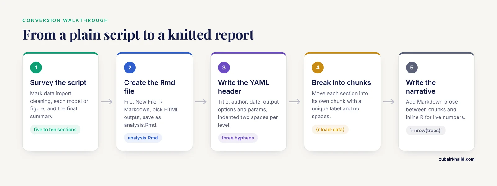
Step 1. Survey the script and find its natural sections

Read the script and mark the places where a reader would want a sentence of explanation: data import, cleaning, each model or figure, and the final summary. Most scripts of a few hundred lines split naturally into five to ten sections. Each section will become one code chunk. If a script has no comments at all, add them first, because those comments become your first draft of the narrative text.

Step 2. Create the R Markdown file

In RStudio, choose File, New File, R Markdown, pick HTML output, and click OK. RStudio creates a template file. Save it as analysis.Rmd in the same project folder as your script, ideally using File, Save As so the working directory is correct. If you prefer the console, run:

rmarkdown::draft("analysis.Rmd", template = "html_document", package = "rmarkdown")

Step 3. Write the YAML header

The lines between the two triple-dashed fences at the top of the file are the YAML header. YAML is a simple indentation-based format for document metadata. A practical header looks like this:

---
title: "Seedling Height Analysis"
author: "Your Name"
date: "`r Sys.Date()`"
output:
  html_document:
    toc: true
    number_sections: true
    code_folding: hide
params:
  data_file: "data/seedlings.csv"
---

The params block defines parameters you can change at knit time with rmarkdown::render("analysis.Rmd", params = list(data_file = "data/other.csv")), which lets one report serve several datasets. Indentation matters in YAML. Every nested option sits two spaces deeper than its parent, and the fence lines must be exactly three hyphens.

Step 4. Break the script into chunks

A code chunk starts with a fence line containing {r} and ends with a fence of three backticks. Move each section of your script into its own chunk and give every chunk a unique label:

trees <- read.csv(params$data_file)

summary(trees$height_cm)

Chunk labels must be unique across the document and should contain no spaces or non-ASCII characters. If two chunks share a label you will meet the duplicate label error described later. Labels are worth the small effort because error messages and the cached-figure system refer to chunks by name.

If your script is long, a quick mechanical approach is to paste the whole thing into one big chunk and then split it at the comment lines. RStudio also has a shortcut: with the cursor in a script file, Code, Insert Chunk (Ctrl+Alt+I on Windows and Linux, Cmd+Option+I on macOS) inserts an empty chunk wherever you are typing.

Step 5. Write the narrative between chunks

This is the step that turns a script into a report. Between chunks, write ordinary Markdown: a short sentence saying what the chunk does and, where relevant, why. Inline R results drop into that prose with backtick-r syntax, for example:

The dataset contains `r nrow(trees)` seedlings measured across
`r length(unique(trees$treatment))` treatments.

When knitted, those inline expressions evaluate to real numbers from the data. The mean you quote in a sentence is computed live, so it cannot drift out of sync with the table beside it.

Step 6. Set chunk options deliberately

Chunk options are comma-separated settings in the braces of the chunk header. The default is to echo the code, evaluate it, and print all output. For a report you usually want to adjust a few. Here is the model section with options:

fit <- lm(height_cm ~ treatment, data = trees) summary(fit)

Setting warning=FALSE is a choice, not a default. Warnings are often meaningful, such as a dropped row from a join or a non-integer count in a Poisson model, so suppress them only when you understand and have addressed them. A compact way to set defaults for the whole document is a hidden setup chunk as the first chunk:

knitr::opts_chunk$set(echo = TRUE, fig.width = 6, fig.height = 4)

Individual chunks can then override any of these values.

Step 7. Knit the document

Click the Knit button in RStudio or run:

rmarkdown::render("analysis.Rmd")

Knitting launches a fresh R session, runs every chunk in order from top to bottom, captures the output, and hands everything to pandoc, the document converter that produces the final HTML, PDF, or Word file. The first knit is the honest test of your analysis. Because the session is fresh, every object must be created by code that appears above the line using it.

Expected output for the example is an HTML file named analysis.html in the same folder, opening in the RStudio viewer pane, showing the title, your prose with live numbers filled in, the code and its printed output, and the boxplot.

Step 8. Verify the result

Check three things. First, scroll the report and confirm every figure and table appears where the prose says it should. Second, confirm that any number quoted in a sentence matches the output it came from, which it will if you used inline R expressions rather than typing numbers. Third, close RStudio, reopen it, and knit again from scratch. If the second knit succeeds, your document is self-contained. If it fails, something in the original script depended on objects from an old session, and the error message will name the missing object.

Step 9. Parameterize and reuse

With the params block from Step 3, the same document can be rendered for many inputs:

rmarkdown::render("analysis.Rmd",
                  params = list(data_file = "data/seedlings_2025.csv"),
                  output_file = "report_2025.html")

This is how a one-off analysis becomes a repeatable pipeline. Teaching resources built this way demonstrate the pattern at scale, showing executable workflows that run from raw data files to final annotated results within a single knitted document [1].

Step 10. Put the source under version control

Commit the .Rmd file, not the knitted .html, to Git. The .Rmd is the human-readable source of truth. Knitted outputs can be regenerated on demand, and committing large binaries bloats repositories. If collaborators need the HTML, render it in a continuous integration job or share it separately.

Chunk Options Reference

A caution on cache=TRUE: a cached chunk does not rerun when the functions it calls change, only when its own code or knit settings change. Add cache.extra = file.mtime(params$data_file) to a cached import chunk so it invalidates when the data file changes. When in doubt, delete the *_cache folder and knit fresh.

Exact Errors and How to Fix Them

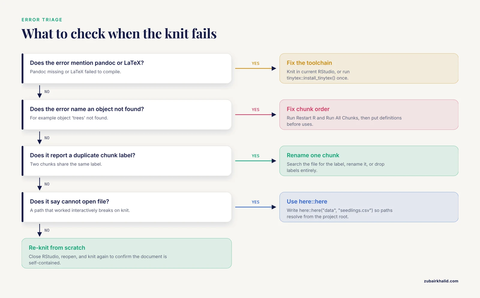
"pandoc version 1.12.3 or higher is required and was not found." RStudio bundles pandoc, so this error usually means you are knitting from plain R or an unusual installation path. Open the project in current RStudio, or install pandoc directly and confirm R can find it with rmarkdown::pandoc_version().

"object 'trees' not found." A chunk uses an object created in a chunk that does not run above it, often because you reordered chunks while experimenting. Run every chunk in order with the Run, Restart R and Run All Chunks command, then fix the ordering so definitions precede uses.

"Duplicate chunk label: 'model'." Two chunks carry the same label. Search your file for the label and rename one, or leave labels off entirely and let knitr assign automatic ones.

"cannot open file 'data/seedlings.csv': No such file or directory." Knitting runs in the directory containing the .Rmd file, not the directory where you last set the working directory interactively. Use the here package and write here::here("data", "seedlings.csv") so paths resolve from the project root regardless of where the knit starts.

"LaTeX failed to compile" when knitting PDF. You have no LaTeX distribution installed. Run tinytex::install_tinytex() once, restart RStudio, and knit again. Small missing LaTeX packages then install automatically on demand.

"YAML block failed to parse" or a blank title. Indentation is wrong, a colon is missing, or a fence is malformed. Every key under output: needs two leading spaces, and unquoted values containing colons must be quoted.

Common Mistakes and Limitations

The most common mistake in converting an R script to R Markdown is assuming chunks run in the order you last executed them. They do not. Knitting runs chunks in document order from a fresh session. Code that references an object defined further down the file will fail, and code that silently depends on variables left over from your interactive session will produce different results or errors. Restart-and-run-all is your friend throughout editing, not just at the end.

A second mistake is suppressing messages and warnings globally from the start. A dplyr join warning or a dropped-factors message in a model summary often signals a data problem worth fixing, and hiding it to make the report pretty hides a bug. Suppress selectively, chunk by chunk, after reading each message.

A third is relative paths that work interactively but break on knit. Set everything through the project root with here::here() or rmarkdown::render() from the project directory, and never leave setwd() in a report, because it encodes your personal folder layout and breaks on any other machine.

A fourth is embedding absolute personal paths, package installations, or hard-coded numbers copied from a previous run into the narrative. Package installation belongs in a separate setup script or renv, not in the report body. Numbers in prose should always come from inline R expressions so they update when the data changes.

Finally, remember the limits of the format. Knitting proves your code runs in order on your machine. It does not prove your statistical model is appropriate, your data are correct, or your interpretation is sound, and a beautifully knitted report is not by itself a deposited, citable artifact. The metabolomics educational review cited earlier makes the point that reproducible analysis requires the whole chain, from raw archived data through scripts to documented workflows, and that document-level literate programming is one layer of that stack rather than the whole answer [1].

A Practical Reproducibility Checklist

Run through this list every time you finish a report. It condenses the practices above into a form you can keep next to your keyboard, and it mirrors the spirit of community checklists used in fields that have formalized analysis sharing [1].

1. The report knits from a fresh R session with Restart R and Run All Chunks.
2. Every package is loaded inside the document with library(), and package versions are recorded, for example with sessionInfo() printed in a final chunk.
3. All file paths resolve with here::here() or parameters, and no setwd() appears anywhere.
4. No number in the prose was typed by hand. Every figure quoted in text uses inline R expressions.
5. Random processes set a seed with set.seed() so results are identical on re-run.
6. Warnings and messages are suppressed only where they were read and understood.
7. The .Rmd source is committed to version control, and the knitted output is regenerated rather than edited by hand.
8. The input data are archived in a public repository where appropriate, so the report can be re-run by someone who is not you.

Frequently Asked Questions

Can I convert an R script to R Markdown automatically?

Yes, partially. The knitr function knitr::spin("analysis.R") converts a specially commented script into an .Rmd file. Lines starting with #+ become chunk options, and normal comments become prose. Spin is a good starting point, but you will still want to split large chunks and edit the narrative by hand.

What is the difference between R Markdown and Quarto?

Both are literate programming systems built on pandoc and knitr. Quarto is the newer, language-agnostic successor that Posit now recommends for new projects, and it uses .qmd files with nearly identical chunk syntax. The conversion steps in this article apply to both, and existing .Rmd files often render in Quarto with minimal changes.

Why does my report fail to knit even though the script runs fine?

The script runs inside your interactive session, which contains objects, loaded packages, and a working directory set by your earlier clicks. Knitting starts a fresh session with none of that. The error message names the first missing piece, usually an object created out of order or a file path relative to the wrong directory.

How do I hide code but keep the output in my report?

Use the chunk option echo=FALSE, which runs the code and shows its output without displaying the code itself. For reports where readers can opt in to seeing code, set code_folding: hide in the html_document options, which collapses code into expandable sections.

How do I make my figures a specific size?

Set fig.width and fig.height in the chunk header, in inches, and set dpi=300 for print-quality resolution. A chunk header such as {r plot, fig.width=6, fig.height=4, dpi=300} produces a six-by-four-inch figure at 300 dots per inch.

Should I commit the knitted HTML file to Git?

Generally no. Commit the .Rmd source and regenerate the HTML on demand, because binary outputs bloat repository history and invite manual edits that drift from the source. Some teams commit rendered output for landing pages or non-technical stakeholders, in which case render it automatically in continuous integration rather than by hand.

How do I share a report with someone who does not use R?

Knit to HTML and send the file, or publish it through Posit Connect, GitHub Pages, or RPubs. The recipient sees the complete report, including code if you left echo=TRUE, in a browser with nothing to install. Word and PDF output formats serve audiences who need print or editable documents.

What is the fastest way to add a new chunk while writing?

Press Ctrl+Alt+I on Windows and Linux, or Cmd+Option+I on macOS, with the cursor in the R Markdown file. RStudio inserts an empty code chunk at the cursor. You can also type the fences manually, but the shortcut avoids the most common syntax slip, which is unbalanced backticks around the chunk header.

Sources

1. Metabonaut: an open educational resource for learning reproducible, script-based untargeted LC-MS/MS metabolomics.