Lab Report Example for Bioinformatics

Q: What sections should a bioinformatics lab report include?

Use the standard seven sections: title, abstract, introduction, methods, results, discussion, and conclusion, plus a reproducibility statement and appendix. The methods section must contain every command, parameter, software version, and reference build so another person can re-run your analysis.

Q: How is a bioinformatics lab report different from a wet-lab report?

The structure is identical, but methods describe code, parameters, and file formats instead of reagents and volumes. Reproducibility is the central requirement, so versions and parameter values carry the weight that reagent lot numbers carry in a wet lab.

Q: How long should a bioinformatics lab report be?

Long enough for full reproducibility and short enough to read in one sitting. For a course report, three to six pages of prose plus tables and an appendix command log is typical. Precision matters more than length.

Q: Do I need to include my actual code and commands?

Yes. Every analysis command belongs in Methods or the appendix, with all flags shown. If you used a script or workflow manager, include the script file or its repository link in the appendix.

Q: Which software versions do I report?

Report the exact version string each tool prints, for example samtools 1.19.2 or GATK 4.4.0.0, plus the reference genome build and the annotation database release. Update the versions if you change anything mid-project.

Q: How do I report variant findings?

Summarize counts first (raw, filtered, by consequence class), then present variants of interest in a table with chromosomal position, gene, consequence, genotype, depth, population frequency, and pathogenicity predictions. Interpretation goes in the Discussion, not the Results table.

Q: Can I reuse a bioinformatics lab report example template?

Yes, a template saves time and enforces consistency. Fill every bracketed field with your own data, delete sections that do not apply rather than leaving them empty, and check any course- or journal-specific requirements before submission.

Q: How should I handle human genomic data in a lab report?

State the data source, the consent that covers it, and where files were stored and processed. De-identify sample names, never include direct identifiers, and note any data-protection rules that constrained your analysis.

By Dr. Zubair Khalid, DVM, MS, PhD · 2026-11-11

By the end of this article you will be able to write a complete bioinformatics lab report, from title page to appendix, for a real analysis: calling variants from human whole-exome sequencing data. You will see the full lab report format, a filled-in example report you can adapt, the exact commands that produced the results, and a reusable template you can copy for your own projects.

To follow the walkthrough on your own computer you need a Unix-like terminal (Linux, macOS, or Windows Subsystem for Linux), Conda or Miniconda for installing tools, and roughly 16 GB of RAM. Everything shown here uses free, open-source software and publicly available reference data.

What Makes a Bioinformatics Lab Report Different

A bioinformatics lab report follows the same skeleton as a wet-lab report, but the "methods" section describes software, parameters, and file formats instead of reagents and pipetting. The reader should be able to re-run your analysis from your methods alone and get the same numbers. That reproducibility requirement shapes every section:

You report exact software versions, not just tool names.
You report every parameter, reference genome build, and database version.
You report file formats and checksums for key outputs, so a reviewer can verify that the files you analyzed are the files you claim to have analyzed.
You separate what the pipeline produced (results) from what it means (discussion).

Standardized headings matter for a second reason as well. When the College of American Pathologists built a recommended heading structure for autopsy reports, the stated goals were consistent organization, easier review by third parties, and easier searching of stored reports [1]. Those same three goals apply to bioinformatics reports. A predictable section structure lets a supervisor, reviewer, or collaborator find your variant counts or your quality-control summary without reading the whole document.

The Standard Lab Report Format, Adapted for Bioinformatics

The classic lab report format has seven core sections. Here is how each one translates to a computational analysis.

Title and identifiers. A descriptive title, your name, date, sample IDs, and the project or accession number if the data comes from a repository.
Abstract or summary. Five to eight sentences stating the question, the data, the main pipeline steps, and the headline result.
Introduction. The biological question, background literature, and a one-sentence statement of what the analysis will do.
Methods. Data source, hardware and software environment, every command with parameters, and the reference databases used.
Results. Tables and figures generated by the pipeline, presented without interpretation. Quality-control metrics, alignment statistics, variant counts, and annotated findings belong here.
Discussion. What the results mean biologically, how confident you are, what could bias the numbers, and what you would do next.
Conclusion and references. A short restatement of the finding, followed by cited literature and tool citations.

Many courses add two more sections that are especially valuable in bioinformatics: a Reproducibility statement (how someone else re-runs your work) and an Appendix with full command logs.

A Worked Example: Whole-Exome Variant Calling Report

This is the core of the article. We will build a report for a realistic scenario modeled on published teaching exercises: sequencing DNA to identify variants that might explain an observed phenotype, then summarizing the findings in a genetic report. A hands-on program at one medical school did exactly this for anatomy cadavers, isolating DNA, running whole-exome sequencing, and producing illustrative clinical genetic reports that students discussed in relation to each donor's cause of death and anatomical findings [2]. Exome sequencing targets the protein-coding fraction of the genome, which contains a disproportionate share of known disease-associated variants, and its workflow runs from DNA extraction through library preparation, target enrichment, sequencing, and computational analysis [3].

Step 1: Set Up the Environment and Define the Question

First, record your software environment. Install tools with Conda:

conda create -n exome-report -c bioconda -c conda-forge \
  fastqc fastp bwa samtools picard gatk4 ensembl-vep
conda activate exome-report

Then capture versions for your Methods section:

bwa 2>&1 | grep Version
samtools --version
gatk --version

Expected output looks like this:

Version: 0.7.17-r1188
samtools 1.19.2
The [Genome Analysis](/blog/guides/genome-analysis) Toolkit (GATK) v4.4.0.0

Copy these exact version strings into your report. "BWA-MEM was used" is not enough. "BWA-MEM version 0.7.17-r1188 was used" is.

The question for this example: Which protein-coding variants does this sample carry in a targeted 40-megabase exome capture region, and do any of them affect genes connected to the observed phenotype?

Step 2: Quality Control on the Raw Reads

Starting from two FASTQ files from an Illumina run, first check read quality:

fastqc sample_R1.fastq.gz sample_R2.fastq.gz -o qc/

Expected output is a set of HTML reports. Inside each one you get a module-by-module summary, for example:

>>Basic Statistics        pass
>>Per base sequence quality  pass
>>Per sequence GC content    pass
>>Sequence Duplication Levels warn

A "warn" is not automatically a problem. High duplication is expected when the input DNA amount is low. Note it and move on, but record it in your Results.

Next, trim low-quality ends and remove adapters:

fastp -i sample_R1.fastq.gz -I sample_R2.fastq.gz \
  -o trimmed_R1.fastq.gz -O trimmed_R2.fastq.gz \
  --qualified_quality_phred 20 --length_required 50 \
  -j fastp.json -h fastp.html

The JSON summary gives you the numbers to quote in your report:

{
  "summary": {
    "before_filtering": { "total_reads": 101371412, "total_bases": 30419342336 },
    "after_filtering":  { "total_reads": 98522304,  "total_bases": 29287314456 }
  }
}

In this example, about 97 percent of read pairs survived filtering. Your Methods section now reads: "Reads were trimmed with fastp version 0.23.4 using a minimum base quality of Phred 20 and a minimum length of 50 bases."

Step 3: A Worked Coverage Calculation

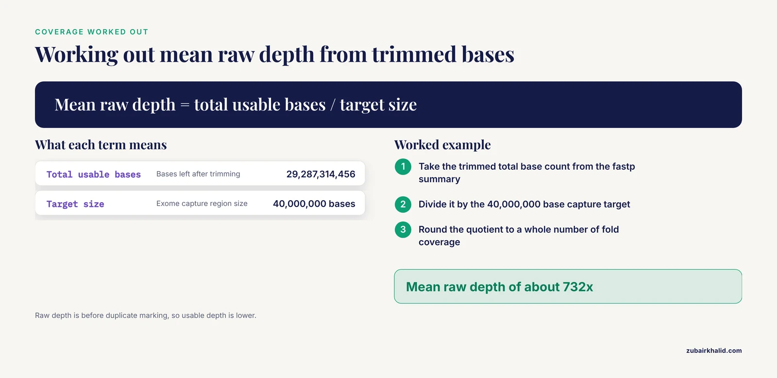
Calculation of mean raw sequencing depth by dividing 29,287,314,456 usable bases by a 40,000,000 base target, giving about 732x.

This calculation belongs in your Results because it tells the reader whether the data can even support variant calling. Say the exome capture targets 40 megabases (Mb) of the genome and the trimmed dataset contains about 29.3 billion bases.

Total usable bases      = 29,287,314,456
Target size             = 40,000,000 bases
Mean raw depth          = 29,287,314,456 / 40,000,000 ≈ 732x

A mean depth of several hundred fold before duplicate removal is typical for clinical-grade exomes. Why depth matters: variant callers distinguish true heterozygous variants (about half the reads show the alternate base) from sequencing errors (a small fraction of reads). At 30-fold depth you can make that distinction with confidence. At 5-fold depth you often cannot. State your achieved depth explicitly so the reader can judge the evidence for every call.

Step 4: Align Reads to the Reference Genome

Align the trimmed reads to the GRCh38 human reference:

bwa mem -t 8 \
  -R '@RG\tID:exome_run1\tSM:sample01\tPL:ILLUMINA' \
  GRCh38.fa trimmed_R1.fastq.gz trimmed_R2.fastq.gz > aligned.sam

samtools sort -@ 8 -o sorted.bam aligned.sam
samtools index sorted.bam

Two parameters deserve explanation in your report. The -t 8 flag sets the number of processor threads, which affects speed but not results. The -R read-group string is more consequential: SM:sample01 tags every read with its sample name. If you omit it, downstream GATK tools will fail with an error, which brings us to common failures.

Error you will actually see. Running GATK HaplotypeCaller on a BAM with no read groups produces:

A USER ERROR has occurred: Argument sampleNameMap has a bad value:
No read groups found in BAM file

Fix: add the -R '@RG\tID:...\tSM:...' argument to bwa mem and realign. The fix costs one re-run, which is why the read group belongs in your Methods section even though it looks like trivia.

Check alignment quality:

samtools flagstat sorted.bam

Expected output:

101371412 + 0 in total ...
96534232 + 0 properly paired (95.21% : N/A)
...

For a healthy exome run you want roughly 95 percent or more of reads mapped and properly paired, with mapped percentage in the high 90s. The unmapped remainder is mostly reads from regions absent from the reference or the capture design, not a sign of failure.

Step 5: Mark Duplicates and Call Variants

PCR duplicates, identical reads that arise from amplification rather than independent fragments, can inflate apparent depth and create false variant calls. Mark them:

picard MarkDuplicates \
  I=sorted.bam O=dedup.bam M=dup_metrics.txt \
  REMOVE_DUPLICATES=false CREATE_INDEX=true

Now call variants within the capture target regions defined in a BED file:

gatk HaplotypeCaller \
  -R GRCh38.fa -I dedup.bam -L targets.bed \
  -O raw_variants.vcf

The output is a VCF (Variant Call Format) file. Each record lists a chromosome, position, reference base, alternate base, genotype, and quality score. A typical record looks like:

chr7    117530967    .    G    A    1245.77    .    DP=89
GT:AD:DP:GQ:PL   0/1:44,45:89:99:1274,0,1361

Read this line as: on chromosome 7 at position 117530967, the sample carries a G-to-A change, with 89 reads of coverage split 44 reference and 45 alternate, a genotype of heterozygous, and a genotype quality of 99 on a Phred scale.

Filter with the hard filters GATK documents for exome data, applied separately to SNPs and indels:

gatk VariantFiltration -R GRCh38.fa -V raw_variants.vcf \
  --filter-name "QD2" --filter-expression "QD < 2.0" \
  --filter-name "FS60" --filter-expression "FS > 60.0" \
  --filter-name "MQ40" --filter-expression "MQ < 40.0" \
  -O filtered_variants.vcf

QD (Qual By Depth) is the variant quality normalized by read depth. FS (Fisher Strand) measures strand bias, the tendency of an artifact to appear on only one strand. MQ (Mapping Quality) is the average alignment quality of supporting reads.

Step 6: Annotate and Interpret

GATK, FreeBayes, DeepVariant, and Platypus are the computational tools commonly compared for exome variant calling, and rigorous quality control plus orthogonal validation are the standard strategies for improving accuracy [3]. Once you have high-confidence calls, annotate them to find out what they do:

vep -i filtered_variants.vcf \
  --cache --assembly GRCh38 --everything \
  -o annotated_variants.vcf

Ensembl VEP (Variant Effect Predictor) adds gene names, consequence types (missense, nonsense, splice-site), pathogenicity predictions, and population frequencies from gnomAD to each variant.

Your Results section then summarizes counts:

Raw variants called:            41,712
Passed hard filters:            33,208
Missense variants:              11,940
Loss-of-function variants:         962
Rare (gnomAD AF < 0.001):        4,201
Variants in phenotype-relevant
genes carried forward:               7

Interpretation happens in the Discussion, and this is where reporting discipline matters most. One published SMA case shows why. A patient with two copies of the SMN1 gene, who would appear unaffected on standard copy-number testing, actually carried a homozygous missense variant in the gene's YG-box domain that disrupted protein function. Initial exome sequencing and deletion analysis both missed it, and only full-length SMN1 sequencing confirmed the diagnosis [4]. The lesson for your report is stated in one sentence: a clean pipeline does not guarantee a correct biological answer, so discuss which variant classes your method can miss.

Step 7: Assemble the Report

Now convert the pipeline log into prose. Here is a filled-in excerpt showing the style, using the numbers generated above:

Methods (excerpt). DNA from sample01 was sequenced on an Illumina platform with paired-end 150-base reads, targeting a 40 Mb exome capture design. Reads were quality-checked with FastQC 0.12.1 and trimmed with fastp 0.23.4 (minimum Phred quality 20, minimum length 50). Trimmed reads were aligned to GRCh38 with BWA-MEM 0.7.17, sorted and indexed with samtools 1.19.2, and duplicate-marked with Picard 3.1.1. Variants were called with GATK 4.4.0.0 HaplotypeCaller restricted to the target BED file and filtered using hard filters (QD < 2.0, FS > 60.0, MQ < 40.0). Variants were annotated with Ensembl VEP release 111.

Results (excerpt). Of 101,371,412 raw read pairs, 97.2 percent survived trimming. Alignment achieved 95.2 percent properly paired reads. Mean raw depth over target regions was approximately 732-fold. Variant calling produced 41,712 raw variants, of which 33,208 passed hard filters. Seven variants in phenotype-relevant genes were carried forward for interpretation.

Discussion (excerpt). The candidate variant in gene X is a rare missense change predicted deleterious by two in silico tools. Interpretation is limited by the absence of parental samples for segregation analysis and by the known blind spots of exome sequencing, which does not capture deep intronic or structural variation [3].

That is the full pattern. Every sentence in Methods traces to a command you ran, and every number in Results traces to an output file.

A Reusable Bioinformatics Lab Report Example Template

Copy this skeleton for your own write-ups. It works for coursework, rotation projects, and first manuscripts.

1. Title, author, date, sample IDs, data accession numbers
2. Abstract (5-8 sentences)
3. Introduction
   3.1 Biological question and background
   3.2 Aim of this analysis (one sentence)
4. Methods
   4.1 Data source and sample description
   4.2 Hardware and software environment (OS, Conda env, versions)
   4.3 Pipeline commands with all parameters
   4.4 Reference genome build and annotation database versions
5. Results
   5.1 Quality control (tables, per-module pass/warn/fail)
   5.2 Alignment and coverage metrics
   5.3 Variant counts and filtering summary
   5.4 Annotated variants of interest (table)
6. Discussion
   6.1 Biological interpretation
   6.2 Confidence and caveats
   6.3 Next steps (validation, follow-up analyses)
7. Conclusion
8. Reproducibility statement (how to re-run: commands, container, seed)
9. References
10. Appendix: full command log, checksums of key files

If your analysis has a spatial or modeling component, the same skeleton still holds. One recent tool, BIWT, embeds single-cell and spatial multi-omics data into agent-based models of virtual tissue, and its authors published both the software on GitHub and the full instructions for reproducing their use-case example [5]. Notice that the reproduction package is part of the contribution, not an afterthought. Your report should aim for the same standard.

Key Parameters and Options at a Glance

Parameter	Tool	What it controls	Typical setting	Where to report it
`-qualified_quality_phred`	fastp	Minimum base quality to keep a base	20	Methods, trimming step
`-length_required`	fastp	Minimum read length after trimming	50	Methods, trimming step
`-R '@RG...SM:...'`	bwa mem	Read group with sample name	One per sample	Methods, alignment step
`-L targets.bed`	GATK HaplotypeCaller	Genomic intervals to call variants	Capture design BED	Methods, variant calling
`QD < 2.0`	GATK VariantFiltration	Quality normalized by depth	SNP and indel hard filter	Methods, filtering step
`FS > 60.0`	GATK VariantFiltration	Strand bias cutoff	SNP hard filter	Methods, filtering step
`-filter-expression "DP < 10"`	VariantFiltration	Minimum read depth per site	Low-depth removal	Methods, filtering step
`-assembly GRCh38`	VEP	Reference genome build for annotation	Must match your FASTA	Methods, annotation step

The single most common reporting failure is a genome build mismatch. Aligning to GRCh38 and annotating against a build-37 database produces shifted coordinates and nonsense gene assignments. Always name the build in both the alignment and annotation steps.

Checking That Your Result Is Right

Before you hand in or submit, run these checks:

Sanity-check the alignment. Properly paired percentage above roughly 95 percent, low adapter contamination after trimming, and per-base quality curves that stay above Phred 30 through most of the read.
Check the variant count against expectations. A typical human exome yields on the order of tens of thousands of single-nucleotide variants. If you got 400 or 400,000, something is wrong, most often a genome mismatch or a missing read group.
Check the transition-to-transversion ratio. True human variation shows more transitions than transversions, and an exome callset should sit near a ratio of 3. A ratio near 1 signals a noisy callset.
Spot-check a known variant. If the sample genotype is available, confirm that a known heterozygous site appears as 0/1 in your VCF with balanced allele depths.
Verify reproducibility. Re-run your pipeline from the top in a fresh directory. The variant counts should match exactly for deterministic tools.

Where Bioinformatics Reports Intersect Clinical Reporting

If your analysis feeds a clinical or diagnostic document, the report structure changes again. Recent work on automated extraction of operative report fields with large language models, for example, evaluated models by how accurately they populated predefined report fields, scoring them with F1 measures against expert annotations, and baseline scores near 0.85 improved to about 0.90 after refinement strategies [6]. The parallel for your own writing is that report quality is measurable against a defined field structure, which is another argument for the standardized template above.

Human genomic data also carries obligations that wet-lab data does not. Genomic data sets are subject to strict data-protection regulation, and privacy-enhancing approaches such as federated learning, differential privacy, and secure multiparty computation are actively studied as ways to analyze such data across institutions while addressing legal constraints like those in the GDPR [7]. A bioinformatics lab report on human data should therefore state where the data came from, what consent covers it, and where the files were stored and processed. That statement takes two sentences and belongs in Methods.

Common Mistakes and Limitations

Missing software versions. Reviewers cannot reproduce "GATK was used." Record the version string from the tool itself, every time.
Reporting results without parameters. A variant count means nothing without the filter thresholds that produced it. The number 33,208 is only meaningful next to QD < 2.0, FS > 60.0, and MQ < 40.0.
Conflating raw depth with usable depth. After duplicate marking and target-capture losses, usable depth is lower than the raw figure. Report both.
Treating in silico predictions as diagnoses. Predicted-deleterious annotations are hypotheses. Published diagnostic work routinely shows discordance between computational calls and clinical truth, as in the SMN1 case where standard testing failed and full-length sequencing was required [4].
Ignoring the reads that did not align. Unmapped reads can carry real biology. At minimum, quantify them rather than deleting them silently.
No negative controls. If your dataset includes a reference sample such as NA12878, run it through the pipeline and compare against its truth set. If it does not, say so as a limitation.
Overstating the conclusion. A variant associated with elevated disease risk is not a diagnosed disease. Precision-medicine teaching programs frame their reports as illustrative and discuss both the potential and the limits of the approach for exactly this reason [2].
No record of failures. The read-group error above, the crashed sort that filled the disk, the wrong BED file. Real methods sections contain the path you actually took, and the failures are often the most useful information for the next person.

For individual clinical questions, a qualified clinician or genetic counselor must interpret any variant finding in context. A lab report, however well written, is not patient care.

Frequently Asked Questions

What sections should a bioinformatics lab report include?