Serial Dilution Calculator: How to Plan and Verify Dilutions
By Dr. Zubair Khalid, DVM, MS, PhD ·

By the end of this guide you will be able to plan a serial dilution from any stock concentration down to a target range, calculate every transfer volume before you pick up a pipette, and verify the finished series with arithmetic and bench checks. The planning stage needs only a serial dilution calculator, a spreadsheet, or the short Python script included below. The verification stage uses tools most teaching and research labs already have, such as a plate reader, agar plates, or the assay you are diluting samples for.
A serial dilution is a chain of dilutions in which each new tube is made from the previous one, so the concentration falls by the same factor at every step. That single idea supports immunoassay standard curves, the calibration curves that relate instrument signal to known concentrations, as well as colony counts in microbiology, antibiotic susceptibility panels, and hook-effect screens that catch falsely low clinical results. Among biology calculators, the serial dilution tool is the one you will reuse most, because the same arithmetic follows you from the teaching lab into research and clinical work, and because dilutions that are never verified fail quietly.
What a Serial Dilution Is and the Words That Describe It
A dilution reduces the concentration of a solution by adding diluent, the liquid used for diluting, usually water, buffer, or culture medium chosen to match the sample. The stock solution is the concentrated starting material. An aliquot is the measured portion moved from one tube to the next. The dilution factor (DF) is the ratio of the concentration before a step to the concentration after it. A 10-fold dilution takes 1000 ng/mL down to 100 ng/mL, and it is made by moving one part sample into a total of ten parts, for example 100 µL into 900 µL of diluent.
A serial dilution chains these steps so each tube becomes the stock for the next tube. The total dilution factor is the product of the per-step factors. Six sequential 10-fold steps dilute the original solution one million-fold (10^6), taking 1000 ng/mL down to 0.001 ng/mL. Ratios carry a naming trap. Most protocols write 1:10 to mean one part sample in ten parts total, which is one part sample plus nine parts diluent, but some older protocols write the same mixture as 1:9. State the actual volumes on your bench sheet so the plan survives the ambiguity.
Serial dilutions exist because they are economical. Each point costs one transfer rather than a fresh weighing and a fresh large volume of stock, and the whole series can be built with one pipette setting. The tradeoff is error propagation, which is the central theme of the verification sections below.
The Math Behind the Plan
Every serial dilution calculator, whether a web form, a spreadsheet, or a script, works with the same five quantities. C0 is the stock concentration. DF is the per-step dilution factor. n is the number of transfers. V_final is the volume you want in each tube. V_transfer is the volume moved at each step. Three relationships generate the whole plan from these.
First, the transfer volume follows from the dilution factor, V_transfer = V_final / DF. The diluent volume in every tube after the first is V_final minus V_transfer. Second, the concentration in tube i is C_i = C_0 / DF^i, where the stock itself is tube 0. Third, the number of steps needed to reach a lowest target concentration C_min is n = ceil(log(C_0 / C_min) / log(DF)), where ceil means round up to the next whole number.
A single dilution that is not part of a chain uses the familiar C_1 V_1 = C_2 V_2. Five milliliters of a 1 M solution diluted to a final volume of 50 mL gives 0.1 M. The serial version applies that same equation repeatedly, with each tube's output becoming the next tube's input.
| Quantity | Formula | Worked example |
|---|---|---|
| Transfer volume per step | V_transfer = V_final / DF | 1000 µL / 10 = 100 µL |
| Diluent per tube | V_diluent = V_final - V_transfer | 1000 - 100 = 900 µL |
| Concentration in tube i | C_i = C_0 / DF^i | 1000 / 10^3 = 1 ng/mL |
| Total dilution factor | DF_total = DF^n | 10^6 over 6 steps |
| Steps needed | n = ceil(log(C_0 / C_min) / log(DF)) | log(10^6) / log(10) = 6 |
| One-step dilution | C_1 V_1 = C_2 V_2 | 5 mL of 1 M to 50 mL gives 0.1 M |
Dilution factors are unitless because concentrations cancel, but the volumes inside each formula must share units. Convert everything to one volume unit before computing, since mixing µL and mL in the same row is a classic failure. The logarithm in the step-count formula is worth internalizing, because equal-ratio steps are the defining feature of a serial dilution and they plot as evenly spaced points on a logarithmic axis. The same log-space reasoning appears in qPCR standard curves and in any bioinformatics calculator that converts between nucleic acid copy number, mass, and molarity, so the habit transfers well beyond the bench.
Using a Serial Dilution Calculator Step by Step
The walkthrough below builds two series that cover the designs you will meet most often, a two-fold standard curve for an immunoassay and a 10-fold chain for a wide dynamic range. Work through the steps once with the example numbers, then substitute your own.
Step 1. Define the stock and the range. Write down the stock concentration and the lowest concentration you need. Example A starts from a 1000 pg/mL top standard and needs points down to about 8 pg/mL. Example B starts from a 1000 ng/mL stock and needs points down to 0.001 ng/mL.
Step 2. Choose the dilution factor. Example A uses a 2-fold factor because the curve needs fine spacing between points. Example B uses a 10-fold factor because the goal is range, not resolution.
Step 3. Compute the number of steps. Apply n = ceil(log(C_0 / C_min) / log(DF)). For Example B:
import math

c0 = 1000.0      # stock concentration, ng/mL
c_min = 0.001    # lowest concentration needed, ng/mL
df = 10          # per-step dilution factor

n = math.ceil(math.log10(c0 / c_min) / math.log10(df))
print(n)
Running the script prints:
6Six transfers produce seven tubes, the stock plus six dilutions. Counting tubes as steps plus one is the most common off-by-one error in planning, so state both numbers explicitly in your plan.
Step 4. Compute the transfer volumes. For 1 mL tubes at a 10-fold factor, V_transfer = 1000 µL / 10 = 100 µL, so each step moves 100 µL into 900 µL of diluent. For Example A, moving 200 µL into 200 µL of diluent gives a 2-fold factor.
Step 5. Build the bench sheet in a spreadsheet. Enter the top concentration once and let the sheet divide:
Cell A2: 1            (tube number, copy down)
Cell B2: 1000         (top standard, pg/mL)
Cell B3: =B2/2        (copy down through B9)
Cell C3: 200          (transfer volume in µL, copy down through C9)
The finished sheet for Example A looks like this:
| Tube | Concentration (pg/mL) | Transfer volume (µL) |
|---|---|---|
| 1 | 1000 | from the stock vial |
| 2 | 500 | 200 |
| 3 | 250 | 200 |
| 4 | 125 | 200 |
| 5 | 62.5 | 200 |
| 6 | 31.25 | 200 |
| 7 | 15.63 | 200 |
| 8 | 7.81 | 200 |
Keep full precision in the spreadsheet, 15.625 and 7.8125, and round only on the printed sheet. Physically, tube 1 holds 400 µL of the top standard, tubes 2 through 8 each start with 200 µL of diluent, and you move 200 µL forward with thorough mixing at every tube. For a 96-well plate, the same formulas apply at smaller volumes. A multichannel pipette with a reservoir keeps every column's transfer identical, and the plate version of Example A moves 100 µL into 100 µL across the columns.
Step 6. Script the whole plan. A short function replaces manual arithmetic and makes the plan reusable:
def serial_dilution(c0, df, n_steps, v_final_ul):
    v_transfer = v_final_ul / df
    v_diluent = v_final_ul - v_transfer
    print(f"Transfer {v_transfer:.0f} uL into {v_diluent:.0f} uL diluent per step")
    print(f"{'Tube':>4}  {'Concentration (ng/mL)':>22}")
    for i in range(n_steps + 1):
        print(f"{i:>4}  {c0 / df ** i:>22.4f}")

serial_dilution(c0=1000.0, df=10, n_steps=6, v_final_ul=1000)
The expected output is:
Transfer 100 uL into 900 uL diluent per step
Tube    Concentration (ng/mL)
   0               1000.0000
   1                100.0000
   2                 10.0000
   3                  1.0000
   4                  0.1000
   5                  0.0100
   6                  0.0010
Step 7. Verify before you pipette. Check that each row satisfies V_transfer + V_diluent = V_final, that the last concentration equals C_0 / DF^n, and that the tube count is n + 1. Then take the plan to the bench and apply the empirical checks in the next section.
Designing the Series: Dilution Factor, Step Count, and Spacing
The dilution factor is a resolution decision. A 10-fold chain covers six orders of magnitude in six tubes, which suits colony-forming unit (CFU) counts, where CFU are the visible colonies descended from individual viable cells and a plate is countable only inside a window of roughly 30 to 300 colonies. You rarely know in advance where an unknown sample will land, so the wide chain finds it. A 2-fold chain resolves concentrations much more finely, which suits minimum inhibitory concentration (MIC) panels, where the MIC is the lowest antibiotic concentration that stops visible growth, and standard curves that must bracket a decision threshold. Three-fold and 5-fold factors are the usual compromise when a 2-fold series would need more tubes than the rack or plate holds.
When the tube count is fixed, solve for the factor instead. Rearranging the step-count formula gives DF = (C_0 / C_min)^(1/n). Covering a million-fold range in six steps gives DF = 10, the classic chain. Covering it in four steps would force a factor near 32, which is awkward to pipette accurately, and that discomfort is the formula telling you to add tubes or make a working stock.
A working stock is a single intermediate dilution, for example 10 ng/mL made from the 1000 ng/mL stock, from which the fine-grained part of the series begins. One extra tube at the top removes several steps at the bottom and cuts the accumulated pipetting error.
Spacing is the other design choice. The standard serial dilution uses equal ratios, so concentrations fall by the same percentage each step. Some engineered systems instead build linear gradients, where concentrations fall by equal absolute amounts, and the two are easy to confuse when you write concentrations into a plan [2]. Decide which spacing your assay expects before you fill tubes, because a curve fit against the wrong spacing produces biased results even when every transfer was perfect.
How to Verify a Serial Dilution
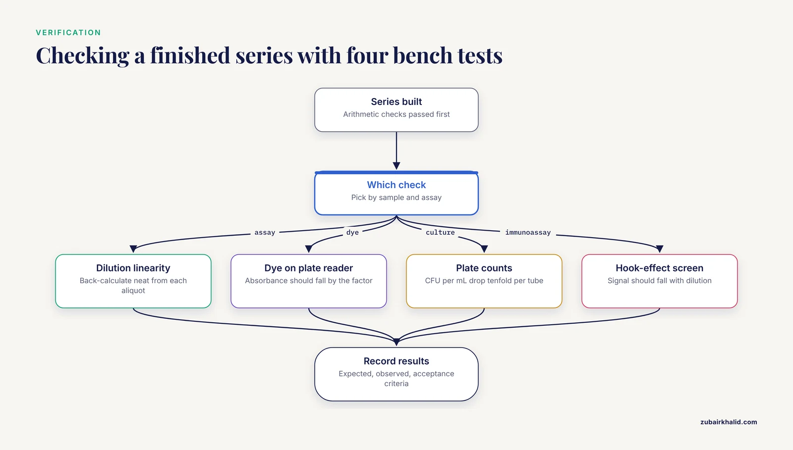
Verification has two layers, arithmetic and empirical. The arithmetic layer takes one minute. Recompute the total dilution factor as DF^n, multiply it through the stock concentration, and confirm the last tube. Confirm every row of the bench sheet satisfies V_transfer + V_diluent = V_final. Confirm the tube count is n + 1. Most planning errors are caught here, before any liquid moves.
The empirical layer asks the tubes themselves. Four standard approaches cover most situations:
- Dilution linearity in the assay itself. Run the neat sample and one or more diluted aliquots, back-calculate the neat concentration from each, and compare. Agreement within the acceptance range stated in the assay insert or your standard operating procedure confirms the series. A universal cutoff does not exist, so use the range your assay documents.
- A dye series on a plate reader. Serially dilute a dye with known absorbance behavior and read each tube. Within the linear range, where absorbance is proportional to concentration (the Beer-Lambert relationship), absorbance should fall by the dilution factor at every step. A step that does not fall proportionally marks a pipetting or mixing failure at that tube.
- Plate counts. For a 10-fold chain of a bacterial culture, CFU per mL should drop tenfold from tube to tube across the countable window. A plateau tells you the culture has reached the detection floor, not that your dilutions failed.
- A hook-effect screen. In a sandwich immunoassay, an extremely high analyte concentration can saturate the capture and detection antibodies separately, so the sandwich complex never forms and the instrument reports a falsely low result. Diluting the specimen stepwise should lower the signal in proportion to the dilution. A signal that instead rises with dilution exposes the hook effect. A 2026 report in Pituitary argues that serial dilution of the specimen, rather than a single fixed dilution protocol, is the appropriate approach for excluding the prolactin hook effect [1]. The same structural logic applies whenever an immunoassay result is implausibly low for the clinical picture.
Whichever check you use, record the expected values, the observed values, and the acceptance criteria on the bench sheet or in your electronic notebook. An unverified dilution and an unrecorded verification are indistinguishable a week later.
What Automation Changes: Lessons From Microfluidic Gradient Generators
Automated dilution does not remove the math, it moves the math into hardware, and a 2026 study in Analytica Chimica Acta shows the parallels clearly [2]. The researchers built a microfluidic chip, fabricated by soft lithography, for rapid parallel testing of antibiotic resistance in biofilms, the structured microbial communities that resist antibiotics far more strongly than free-floating cells. Two syringe pumps delivered lysogeny broth (LB), a standard bacterial growth medium, and gentamicin, an antibiotic, into a multi-stage gradient generator that fed five culture chambers. Each chamber carried interdigitated electrodes, comb-shaped electrode pairs used for electrochemical impedance spectroscopy (EIS), a label-free electrical readout of bacterial growth.
The design details map one to one onto manual dilution concerns. The serial injection mode stacks the two streams into a three-layer fluid structure that doubles the interfacial contact area, so diffusion mixes them without external energy. The connecting-channel width was offset by 125 µm to overcome pressure-gradient dilution, a systematic bias in which pressure differences dilute the stream unintentionally, and the finished device held a stable linear gradient spanning 24.3 to 91.8 percent of a 5 to 18 µg/L gentamicin range [2]. Read that as the fluidic equivalent of pipette calibration. Even a machined chip must measure its own dilution bias and compensate for it, which is exactly what a pipette check does for your hands. The chip also confirms the spacing point above, since its gradient is deliberately linear rather than logarithmic.
Serial Dilution Calculator Tips for the Bench
These habits separate plans that hold from plans that drift:
- Print the plan before pipetting. Label every tube with its target concentration and dilution factor first, then fill. Filling while calculating is where transcription errors enter.
- Use a working stock to shorten the chain. Fewer steps mean less compounded error and fewer transfers.
- Keep transfer volumes in the pipette's accurate range. Very small transfers, well below a tenth of the pipette's maximum, carry the weakest accuracy specifications. Redesign the series with larger volumes rather than trusting them.
- Match the diluent to the sample matrix. Diluting serum into plain buffer changes protein binding and can shift the apparent concentration. Use the matrix the assay expects.
- Mix after every transfer. Pipette up and down several times or vortex briefly. Incomplete mixing biases the next transfer, so the error propagates forward through the chain.
- Change tips between samples that stick or carry over. Viscous solutions cling to tips and carry concentrated material into dilute tubes.
- Include a blank and duplicate the top standard. The blank anchors the zero point, and the duplicate catches a bad first transfer.
- Record the diluent, lot numbers, and pipette identity on the bench sheet. When a series drifts, those entries make the drift traceable.
Once a template survives verification twice, save it as the lab's reference plan with your common dilution factors, volumes, and units already filled in. New members then inherit a verified design instead of reinventing one at the bench.
Common Mistakes and Limitations
Most serial dilution calculator mistakes are planning mistakes, and they appear before the first pipette stroke. The recurring ones, with fixes:
- Confusing the dilution factor with the ratio convention. A 1:10 dilution has a dilution factor of 10 when it means one part sample in ten parts total. A protocol that writes 1:9 for the same mixture is using the other convention. Write volumes, not just ratios.
- Off-by-one tube counts. n transfers produce n + 1 concentrations, because the stock is tube 0. A six-step series fills seven tubes. Plan rack space and diluent volumes for n + 1.
- Transfer volume arithmetic. At a 10-fold factor with 1 mL tubes, the move is 100 µL into 900 µL of diluent. Moving 100 µL into 1000 µL produces a factor of 11 and silently shifts every downstream concentration.
- Pipetting outside the accurate range. A 5 µL transfer from a 1000 µL pipette can be off by a large percentage, and that error then multiplies through every later tube. Change pipettes or redesign the volumes.
- Skipping the mix. An unmixed tube donates a concentrated aliquot forward, biasing everything after it.
- Unit slips. mg/mL and µg/mL differ by 1000. Enter units in the spreadsheet header and keep the cells numeric.
- Wrong spacing. A curve fit assumes the concentrations you wrote. If the plan was logarithmic and the fit assumes linear spacing, or the reverse, the curve is biased even with perfect pipetting.
Calculators also fail in characteristic ways, and the messages are diagnostic. A spreadsheet returns #DIV/0! when the dilution factor cell is blank or zero, because the concentration formula divides by it, and #VALUE! when a concentration cell contains text such as 1,000 ng instead of the number 1000. Keep units in the header row and numbers only in data cells. In Python, math.log10 raises ValueError: math domain error when the stock or target concentration is zero or negative, and a dilution factor of zero raises ZeroDivisionError on the first step past the stock. Both point to the inputs, not the code.
Limitations deserve equal billing. A calculator produces a plan, not a measurement. It assumes calibrated pipettes, complete mixing, a matched diluent, and no evaporation or adsorption of analyte to tube walls, and at small volumes those assumptions strain first. Error also compounds multiplicatively, so the uncertainty in the last tube of a long chain is several times the uncertainty of any single transfer, which is why verification focuses on the dilute end. Finally, calculation is not interpretation. A dilution-corrected clinical result, such as a prolactin value revised after a hook-effect workup, needs review by a qualified laboratory professional before it guides care.
Frequently Asked Questions
What does a serial dilution calculator do?
A serial dilution calculator converts three inputs, the stock concentration, the per-step dilution factor, and the number of steps, into the concentration and transfer volume for every tube in the series. A good calculator also reports the total dilution factor and flags when a target concentration falls outside the range the series can reach.
How do I calculate the concentration in each tube?
Divide the stock concentration by the dilution factor raised to the tube number, C_i = C_0 / DF^i. A 1000 ng/mL stock diluted 10-fold per step gives 100 ng/mL in tube 1, 10 ng/mL in tube 2, and 1 ng/mL in tube 3.
What dilution factor should I choose?
Choose a 10-fold factor when you need to cover a wide concentration range quickly, and a 2-fold factor when you need fine resolution around a threshold such as an assay endpoint. Three-fold and 5-fold factors are common compromises when a 2-fold series would need too many tubes.
How many steps do I need to reach a target concentration?
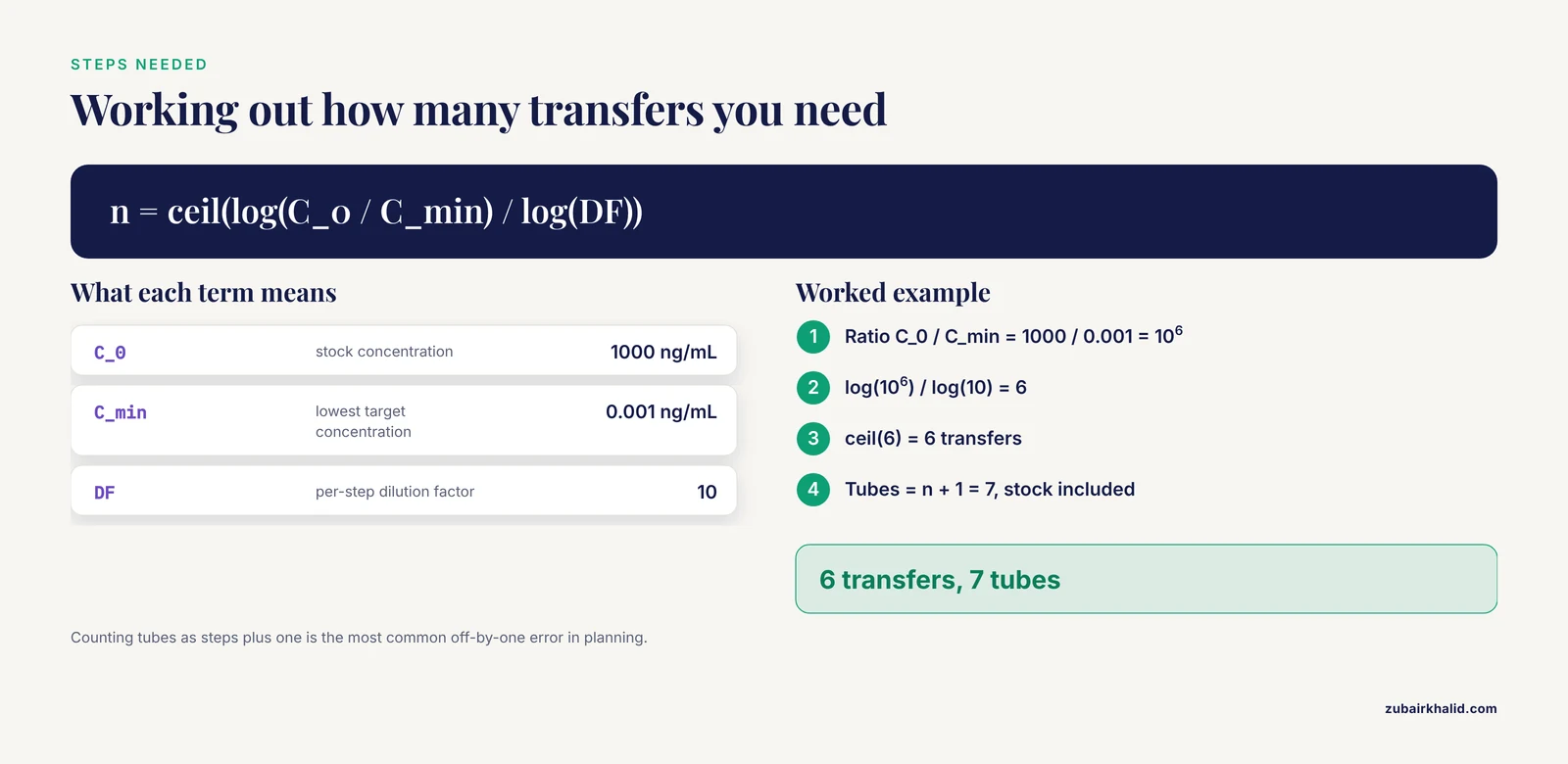 Compute n = ceil(log(C_0 / C_target) / log(DF)). Going from 1000 ng/mL to 0.001 ng/mL at 10-fold per step needs 6 transfers, which produces 7 tubes including the stock.
Is a 1:10 dilution the same as a 10-fold dilution?
Yes, when 1:10 means one part sample brought to ten parts total, which is one part sample plus nine parts diluent. The confusion comes from protocols that write the same mixture as 1:9, so record the actual volumes on your bench sheet.
What is the difference between a serial and a direct dilution?
In a serial dilution each tube is made from the previous tube, while in a direct dilution every working concentration is prepared independently from the stock. Serial dilutions use less stock and fewer pipette settings, and direct dilutions keep an error in one tube from propagating into the others.
Why do my diluted samples drift from the calculated values?
Pipetting error compounds at every step, so the last tubes in a long series drift furthest from the plan. Larger transfer volumes, calibrated pipettes used inside their accurate range, and thorough mixing after every transfer keep the drift small.
How does a serial dilution help detect the hook effect?
In a sandwich immunoassay, an extremely high analyte concentration can saturate both antibodies and return a falsely low result. Diluting the specimen step by step should lower the measured signal in proportion, and a signal that instead rises with dilution exposes the hook effect.