Outlier Detection Calculators for Lab Data: A Practical Guide
By Dr. Zubair Khalid, DVM, MS, PhD ·

By the end of this guide you will be able to take a column of replicate measurements, run four standard outlier tests on it in Python or a spreadsheet, read each output correctly, and make a defensible decision about the flagged value. You will also know when a one-column test is the wrong tool and a domain-specific bioinformatics calculator is the better choice.
Here is what you need on hand:
- A small dataset, ideally 10 to 20 replicate readings of the same sample
- Python 3 with numpy and scipy installed (run
pip install numpy scipy), or any spreadsheet if you prefer no code - A note of your sample size (n) and your significance level (alpha), the false-flag rate you are willing to accept, conventionally 0.05
If you have searched for an outlier detection calculator for biology lab data, you have mostly found single-form web widgets. They compute one formula and stop. The workflow below shows the decisions those widgets hide, which is where the answer actually gets its meaning.
What an Outlier Detection Calculator Does
An outlier is a measurement that lies far outside the pattern formed by the rest of the sample. An outlier detection calculator converts the vague question "does this value look wrong?" into a reproducible number compared against a fixed cutoff.
This matters because bench biology runs on small samples. Pharmacology and experimental biology datasets frequently contain fewer than 20 observations, where a single reading can disproportionately move a mean, a standard deviation, or a significance test, and ad-hoc removal risks replacing the anomaly with investigator bias [1]. Many traditional outlier methods were optimized for large datasets and perform poorly at the sample sizes typical of bench science, which is why the choice of calculator matters as much as the calculation itself [1].
Calculators come in two families:
- Single-variable statistical tests for replicate data, plate readings, and short measurement series. These include Tukey fences, the median absolute deviation z-score, Grubbs' test, and Dixon's Q test. This article walks through all four.
- Pipeline-level detectors for high-throughput data, where outliers are samples, spots, or genomic loci rather than single readings. Modern examples include outlier detection built into cellular impedance workflows [2], deep-learning quality control for quantitative proteomics [3], and median absolute deviation screening for artifacts in spatial transcriptomics [4].
Both families answer the same question with different granularity. The mistakes also carry over, which is why the single-variable tests are worth learning even if your daily work is sequencing.
Matching the Test to Your Data
Four parameters drive the choice of test:
- Sample size (n). Very small samples need tests with critical values built for them.
- Alpha. The significance level, usually 0.05, sometimes 0.01 when an exclusion will change a reportable result.
- Distribution. Grubbs and Q assume approximately normal data. Tukey fences and the MAD z-score do not.
- Number of suspects. One suspicious point calls for a single-outlier test. Several call for a sequential or robust method.
The table summarizes the standard options.
| Test | Statistic and cutoff | Assumptions | Best for | Main weakness | ||
|---|---|---|---|---|---|---|
| , - | , - | , - | , - | , - | ||
| 3 sigma z-score | z = (x - mean)/s, flag if \ | z\ | > 3 | Approximate normality, larger n | Quick screening of large runs | The outlier inflates s and hides itself in small samples |
| Tukey fences | Flag outside Q1 - 1.5×IQR or Q3 + 1.5×IQR | None strict | Any n, distribution-free screening | Flags about 0.7 percent of clean normal points by design | ||
| MAD z-score | 0.6745(x - median)/MAD, flag if > 3.5 | None strict | Contaminated or skewed data | MAD collapses to 0 when many values tie | ||
| Grubbs' test | G = max\ | x - mean\ | /s above a table value | Approximate normality, one suspect | A single outlier for n from about 7 upward | One test per round, repeated rounds inflate false positives |
| Dixon Q test | Q = gap/range above a table value | Approximate normality | Very small samples, roughly n = 3 to 10 | Tests only the single extreme point | ||
| Generalized ESD | Sequential Grubbs with adjusted cutoffs | Approximate normality | Several suspected outliers in larger samples | Needs an upper bound on the number of outliers |
Here IQR is the interquartile range, the span between the 25th and 75th percentiles, and MAD is the median absolute deviation, the median of the absolute distances from the median. The 0.6745 factor makes the MAD directly comparable to a standard deviation under normality, and 3.5 is the conventional flag threshold from the Iglewicz and Hoaglin recommendation.
Step-by-Step: Using an Outlier Detection Calculator on Lab Data
The worked example is a set of ten replicate absorbance readings from a plate-based assay. The last reading is suspiciously high. Every calculation below runs in seconds.
Step 1: Set up the data
import numpy as np
from scipy import stats

absorb = np.array([0.451, 0.462, 0.448, 0.459, 0.455,
                   0.461, 0.449, 0.457, 0.453, 0.612])
n = absorb.size
print(n, round(absorb.mean(), 4), round(absorb.std(ddof=1), 4))
Expected output:
10 0.4707 0.0499The mean is 0.4707 and the sample standard deviation is 0.0499. Keep these two numbers in mind, because the suspect point is already dragging both upward.
Step 2: Screen with Tukey fences
q1, q3 = np.percentile(absorb, [25, 75])
iqr = q3 - q1
low_fence = q1 - 1.5 * iqr
high_fence = q3 + 1.5 * iqr
print(np.round([q1, q3, iqr, low_fence, high_fence], 4))
print(absorb[(absorb < low_fence) | (absorb > high_fence)])
Expected output:
[0.4515 0.4605 0.009  0.438  0.474]
[0.612]
The interquartile range is 0.009, so the fences sit at 0.438 and 0.474. The reading 0.612 falls far above the upper fence. NumPy's default percentile interpolation matches the spreadsheet function QUARTILE.INC, so you should get the same numbers in Excel or Google Sheets.
Step 3: Score with the MAD z-score
med = np.median(absorb)
mad = np.median(np.abs(absorb - med))
robust_z = 0.6745 * (absorb - med) / mad
print(med, mad)
print(np.round(robust_z, 2))
Expected output:
0.456 0.005
[-0.67  0.81 -1.08  0.4  -0.13  0.67 -0.94  0.13 -0.4  21.04]
The median (0.456) barely moved when the suspect point arrived, which is the whole point of a robust summary. The suspect point scores 21.04, far beyond the 3.5 threshold, while every clean reading sits between -1.08 and 0.81. This is the clearest separation of the four methods, because the median and the MAD are barely influenced by extreme values.
Step 4: Confirm with Grubbs' test
Grubbs' test, also called the extreme studentized deviate test, uses the largest absolute deviation from the mean divided by the sample standard deviation. Its critical value accounts for sample size, which the raw 3 sigma rule does not.
mean = absorb.mean()
sd = absorb.std(ddof=1)
dev = np.abs(absorb - mean)
g = dev.max() / sd
t_crit = stats.t.ppf(1 - 0.05 / (2 * n), n - 2)
g_crit = (n - 1) / np.sqrt(n) * np.sqrt(t_crit**2 / (n - 2 + t_crit**2))
print(np.round([mean, sd, g, g_crit], 4))
print("flagged value:", absorb[dev.argmax()])
Expected output (your last decimal may differ slightly):
[0.4707 0.0499 2.8326 2.2898]
flagged value: 0.612
G = 2.83 exceeds the 5 percent critical value of 2.29, so the point is a statistically significant outlier. Some printed tables list 2.18 for n = 10 because they use a different convention for the two-sided alpha. The margin here is wide enough that the verdict does not change, but you should always record which table or function produced your cutoff.
Step 5: Cross-check with Dixon's Q test
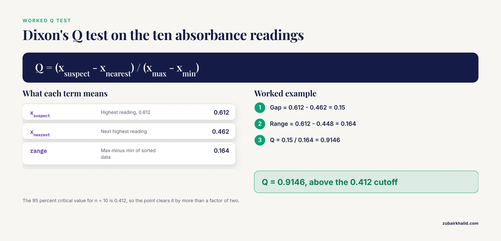
Dixon's Q test is built for very small samples. It divides the gap between the suspect point and its nearest neighbor by the total range of the data.
s = np.sort(absorb)
gap = s[-1] - s[-2]
rng = s[-1] - s
q_stat = gap / rng
print(s)
print(np.round([gap, rng, q_stat], 4))
Expected output:
[0.448 0.449 0.451 0.453 0.455 0.457 0.459 0.461 0.462 0.612]
[0.15   0.164  0.9146]
Q = 0.9146. Standard tables list a 95 percent critical value of 0.412 for n = 10, so the calculated Q clears it by more than a factor of two. The Q test is the small-sample workhorse recommended for objective screening in bench-scale datasets [1].
Step 6: See why the 3 sigma rule fails here
z = (absorb - absorb.mean()) / absorb.std(ddof=1)
print(np.round(z, 2))
Expected output:
[-0.39 -0.17 -0.46 -0.23 -0.31 -0.19 -0.44 -0.27 -0.35 2.83]The largest z-score is 2.83, below the cutoff of 3. The naive rule misses the exact point that three proper tests flagged. In clean normal data of this size, the largest z-score typically lands between 1.5 and 2, so a cutoff of 3 almost never fires. This failure mode is called masking, and it is the single biggest reason to prefer size-aware tests in the lab.
Common errors and their fixes
ModuleNotFoundError: No module named 'scipy'. The scipy package is not installed. Runpip install scipy.NameError: name 'np' is not defined. The import line did not run in the current session. Rerun the import block.RuntimeWarning: divide by zero encountered in dividewithinfin the output. The MAD is 0 because more than half of your values are identical. Switch to Tukey fences, or use the mean absolute deviation from the median as the scale instead.#DIV/0!in a spreadsheet. The standard deviation formula points at an empty or misspelled range. Check the cell range in the formula bar.
How to verify the output
- Recompute one method by hand on the sorted list. The Q test is easiest, since it is one subtraction divided by another.
- Confirm that at least two methods flag the same point. Agreement between a parametric test (Grubbs, Q) and a robust one (MAD, Tukey) is strong evidence.
- Plot the data as a Tukey boxplot with the individual points overlaid, part of the "Visual Trio" approach proposed for small pharmacological datasets, so the statistical verdict and the picture tell the same story [1].
- Check the instrument log for a documented cause such as a pipetting fault, a bubble in the well, or a skipped wash step.
Deciding what to do with a flagged value
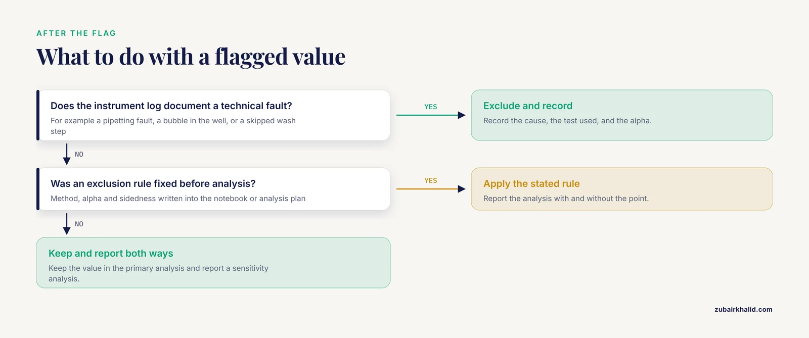
A significant test result means the point is unusual, not that it is wrong. The decision follows a fixed order:
- If the instrument log documents a technical fault, exclude the value and record the cause, the test used, and the alpha.
- If no cause is documented, keep the value in the primary analysis and report a sensitivity analysis with and without it. This both-ways reporting is the standard recommendation for small biological datasets [1], and it mirrors how meta-analysts handle an influential study whose exclusion changes the pooled estimate [5].
- Never exclude a point solely because it weakens the result you wanted.
No-code option: spreadsheet formulas
For the same dataset in cells A2 through A11:
- Quartiles:
=QUARTILE.INC(A2:A11,1)and=QUARTILE.INC(A2:A11,3) - Median and MAD: put
=ABS(A2-MEDIAN($A$2:$A$11))in B2, fill down to B11, then=MEDIAN(B2:B11) - Mean and standard deviation:
=AVERAGE(A2:A11)and=STDEV.S(A2:A11) - Grubbs statistic:
=(MAX(A2:A11)-AVERAGE(A2:A11))/STDEV.S(A2:A11) - Q statistic:
=(MAX(A2:A11)-LARGE(A2:A11,2))/(MAX(A2:A11)-MIN(A2:A11))
Compare the Grubbs and Q results against the table values for your n. This kind of spreadsheet is the simplest biology calculator for outlier work, and it is fully adequate for single-column tests.
Practical Tips for Trustworthy Outlier Calls
- Fix the rule before you look at the data. Write the method, the alpha, and the sidedness into your notebook or analysis plan before running anything. This is the core recommendation of the structured workflow developed for small-sample pharmacological data [1].
- Pair a parametric and a nonparametric test. Plant genomics workflows do exactly this, pairing the parametric 3 sigma rule with the nonparametric Tukey method as complementary filters, so that agreement between the two strengthens the call [6].
- Prefer robust summaries when contamination is likely. MAD-based detection is the screening engine in spatial transcriptomics artifact detection, precisely because medians resist being dragged by the bad regions they are hunting [4].
- Flag in real time for longitudinal data. In wastewater pathogen surveillance built on digital PCR, occasional high outliers bias trend estimates and the epidemic indicators derived from them, and a fast real-time detection method improved the re-estimated trends in the majority of evaluated situations [7].
- Report n before and after exclusion. A result should never force the reader to guess how many points it rests on.
- Match the calculator to the data structure. Impedance time courses, NMR spectra, and sequencing outputs need domain tools rather than a single z-score, as covered in the next section.
Common Mistakes and Limitations
- Trusting the 3 sigma rule in small samples. Masking makes this the most common failure in bench data. The suspect point inflates the standard deviation, which shrinks its own z-score below the cutoff. The walkthrough demonstrated this directly.
- Repeated test-and-remove rounds. Running Grubbs, removing the winner, and running Grubbs again multiplies your chances of flagging a clean point. If you expect several outliers, use the generalized ESD test, which adjusts each sequential cutoff, and declare the maximum number of suspects in advance.
- Running univariate tests across thousands of features. A per-feature test with no multiple-testing control will flag noise. High-dimensional screening is also sensitive to a handful of influential points, and simulation work on epigenome-wide screening shows that influential outliers measurably change which sites are retained [8].
- Ignoring the distribution. Fold changes, cytokine ratios, and many imaging metrics are right-skewed. Log-transform before applying Grubbs or Q, or lean on Tukey fences and the MAD z-score, which carry no normality assumption.
- Confusing biological signal with technical error. In a dose-response series the top dose is supposed to differ. Test for outliers within treatment groups, never across them. Principled exclusions do exist, for example the removal of ancestry-based outliers in genetic association studies to control population stratification, but those follow a stated rule tied to study design [9].
- Deleting points to rescue significance. This is the fastest route to an unreproducible result. Pre-specify the exclusion rule and report both analyses [1].
- Treating the calculator as validation. Small-sample tests have limited power, and deep-learning detectors for proteomics quality control achieve strong performance but still require independent validation before they gate your decisions [3], [10].
- Conflating censored values with outliers. Readings below the detection limit are not outliers. Handle non-detects through prespecified sensitivity analyses rather than post-hoc exclusion [1].
When to Reach for a Bioinformatics Calculator Instead
Once your data becomes a matrix rather than a column, the single-variable tests stop being the right instrument, and the appropriate bioinformatics calculator is a pipeline built for the assay:
- Cellular impedance sensing. The vascr toolkit imports multi-frequency data from multiple instrument manufacturers and includes outlier detection alongside resampling and ANOVA-based testing [2].
- Quantitative proteomics. MCOD processes MaxQuant outputs directly and outperformed 18 statistical, machine learning, and deep learning baselines across simulations and real cancer datasets [3]. MFF-AE is a complementary autoencoder that fuses global and local features of mass spectrometry matrices to identify anomalous samples [10].
- Copy number calling. CNV-ECOD applies empirical-cumulative-distribution-based outlier detection to read depth signals, then refines boundaries with paired-end and split-read evidence [11].
- Selection scans. pyFLANK infers the null distribution for FST (fixation index, a measure of genetic differentiation between populations) outlier detection from quasi-independent loci using a graph neural network, achieving lower false positive rates than existing methods at comparable power [12].
- Repeat expansions. TRoLR built population distributions for over three million tandem repeat loci from 471 ancestrally diverse long-read genomes and flags outlier expansions for clinical prioritization [13].
- Transcriptomic diagnostics. paRDal automates expression outlier detection in parallel RNA and DNA sequencing for hereditary cancer workups [14], and MAJIQ-CLIN identifies outlier splicing events in patient RNA sequencing data [15].
- Spectroscopy and metabolomics. The GNAT toolbox embeds graphical outlier detection tools in a full NMR metabolomics pipeline [16], and automated machine learning frameworks for spectral phenotyping likewise evaluate outlier detection as part of model assessment [17].
The common thread is that each of these tools encodes assumptions about its own data structure. A Grubbs test on 20,000 proteins is not a simplified version of MCOD. It is a category error.
Frequently Asked Questions
What is an outlier detection calculator in biology?
It is a tool that runs a statistical test such as Grubbs, Dixon Q, Tukey fences, or a MAD z-score on your measurements and flags any value that is statistically inconsistent with the rest. Good calculators state the test, the sample size, and the alpha, so the call is reproducible.
Which outlier test works best for a sample size of 5?
Dixon's Q test, because its critical values were built for very small samples. Pair it with a robust method such as the MAD z-score as a cross-check, and avoid the 3 sigma rule entirely at this size.
Can I delete an outlier from my lab data?
Only when you have a documented technical cause or a rule you fixed before analysis. Report the analysis with and without the point so readers can see the effect of the exclusion.
What does a Q value of 0.412 mean?
It is the 95 percent critical value for n = 10. A calculated Q above 0.412 means the extreme point is a statistically significant outlier at the 5 percent level.
Does my data need to be normally distributed for these tests?
Grubbs and Q assume approximate normality, while Tukey fences and the MAD z-score do not. Log-transform skewed measurements such as fold changes before the parametric tests, or use the robust methods directly.
How do I deal with more than one suspected outlier?
Use the generalized ESD test with a declared upper bound on the number of suspects, or a robust method that scores all points at once. Avoid repeated test-and-remove rounds, which inflate the false positive rate.
What significance level should I choose?
Alpha = 0.05 is the conventional default. Choose 0.01 when a flagged value will be excluded from a reportable result, and state the level in your analysis plan before you run the test.
Are free online outlier calculators safe to use for lab records?
They are fine for a quick check if they state the exact test, the sample size, and the cutoff table. For anything that enters a lab notebook or a manuscript, prefer scripted code or a validated pipeline tool so the analysis is reproducible.
Sources
- Beyond bar charts: A practical guide to small sample pharmacological data.
- vascr: An R-based toolkit for rapid and robust analysis of cellular impedance sensing data.
- MCOD: a memory-constrained deep learning framework for robust outlier detection in quantitative proteomics.
- SpatialArtifacts: a computational framework for tissue artifact detection in spatial transcriptomics data.
- Enamel damage from tooth-whitening- a systematic review and meta-analysis.
- Alleleauto: a pipeline for allele identification and analysis of allele-specific gene expression with haplotype-resolved diploid genome assemblies.
- Real-time outlier detection in digital PCR data for wastewater-based pathogen surveillance.
- Impact of influential data on screening epigenome-wide data.
- Genetic Susceptibility Within the Immune System Beyond Conventional Risk Factors: An Integrative Analysis in a Kazakh Cohort.
- MFF-AE: Enhanced Quality Control for Proteomics Mass Spectrometry Data via Multi-Scale Feature Fusion.
- CNV-ECOD: A copy number variation detection method based on ECOD algorithm using next-generation sequencing data.
- pyFLANK, a graph neural network based null distribution inference model for F(ST) outlier detection.
- Genome-wide detection and clinical prioritization of tandem repeat outliers using long-read sequencing.
- paRDal: bioinformatics framework for a parallel RNA and DNA NGS analysis in hereditary cancer diagnostics.
- MAJIQ-CLIN: A novel tool to help identify Mendelian disease-causing variants from RNA-seq data.
- General Nuclear Magnetic Resonance Analysis Toolbox for Stats: A Comprehensive Module for Nuclear Magnetic Resonance-Based Chemometrics and Metabolomics.
- Prediction of Total Anthocyanin Content in Single-Kernel Maize Using Spectral and Color Space Data Coupled with AutoML.