How to Use a Backcross Calculator: Step-by-Step Guide
By Dr. Zubair Khalid, DVM, MS, PhD ·

By the end of this guide, you will be able to use a backcross calculator to compute expected genotype frequencies for any backcross generation, predict how quickly the recurrent parent's genome returns, size a population for a marker-assisted selection target, and test whether your observed segregation counts match theory. You need a spreadsheet, or Python 3 with the scipy package installed for the chi-square step, plus a few numbers from your own cross: the parental genotypes, the number of backcross generations, and recombination fractions if you work with linked markers.
A backcross is a cross between a hybrid and one of its parents, or between a hybrid and an individual genetically similar to that parent. The parent you keep crossing back to is the recurrent parent. The parent supplying the allele (one variant of a gene) you want to capture is the donor parent. The first generation of that cross is called BC1. Each round of backcrossing cuts the donor parent's remaining genome share in half on average, which is why backcrossing is the standard route for moving a single valuable allele into an elite genetic background while restoring everything else.
What a Backcross Calculator Does
A backcross calculator is a biology calculator built around the segregation pattern of repeated backcrossing. A general Punnett square tool answers the question of which genotypes a single cross produces. A backcross calculator answers breeding questions: how much donor genome remains after three generations, how many progeny you must screen to find a plant carrying recurrent alleles at two flanking markers, and whether the 52:48 split you counted in the greenhouse fits the expected 1:1 ratio.
Students use these tools to check linkage problems. Plant breeders use them to plan marker-assisted backcross breeding (MABB), the pipeline that moves a target allele into an elite cultivar with molecular markers guiding each generation [1]. Animal breeders run the same arithmetic to plan how many generations are needed to dilute a donor breed's contribution. When the calculator ingests marker genotype data, such as single nucleotide polymorphism (SNP) calls from a genotyping assay, it crosses into bioinformatics calculator territory, because it is now processing rows of genotype calls rather than a single cross.
Typical inputs are the parental genotypes, the generation number, recombination fractions between markers and the target locus, and observed progeny counts. Typical outputs are genotype frequencies, the expected fraction of recurrent parent genome, minimum population sizes, and chi-square statistics with their degrees of freedom.
The Core Formulas a Backcross Calculator Uses
The table summarizes the formulas that drive almost every backcross calculation. The paragraphs after it explain where each one comes from.
| Calculator output | Formula | Worked example |
|---|---|---|
| BC1 ratio at one locus | 1 heterozygote : 1 recurrent homozygote | 100 BC1 progeny give about 50 carriers and 50 non-carriers |
| Recurrent genome after n backcrosses | 1 - (1/2)^n | n = 3 gives 93.75% |
| Donor genome after n backcrosses | (1/2)^n | n = 3 gives 6.25% |
| Double recombinant proportion in BC1 | (r1 × r2) / 2 | r1 = r2 = 0.10 gives 0.005 |
| Population size for confidence c | ln(1 - c) / ln(1 - p), rounded up | p = 0.005, c = 0.95 gives 598 plants |
| Chi-square goodness of fit | Σ (O - E)² / E | 52:48 against 1:1 gives 0.16 |
| Degrees of freedom | number of classes - 1 | a 1:1 test has df = 1 |
Recurrent parent genome recovery. After n generations of backcrossing to the same recurrent parent, the expected fraction of the genome from that parent is 1 - (1/2)^n. The reasoning is simple: the F1 (first filial generation, the offspring of the initial cross) carries half donor and half recurrent genome, and each backcross replaces half of whatever donor segment remains, on average. This is a population expectation, not a guarantee for any single plant.
Single-locus expectations. A heterozygous F1 (Aa, meaning the two alleles at that locus differ) crossed to a homozygous recurrent parent (aa, meaning both alleles are identical) produces BC1 progeny in a 1 heterozygote to 1 recurrent homozygote ratio. The same 1:1 expectation holds at that locus in every later backcross generation, because selected heterozygotes are again crossed to the homozygous recurrent parent. With two unlinked loci, the BC1 expectation widens to a 1:1:1:1 ratio across four genotype classes.
Double recombinants. A recombination fraction (r) is the proportion of gametes in which a crossover occurred between two loci, ranging from 0 (completely linked) to 0.5 (independent assortment). With the donor allele sitting between two flanking markers in coupling phase (donor alleles on the same homolog in the F1), the proportion of BC1 progeny that carry the donor allele at the target but recurrent alleles at both flanks is (r1 × r2) / 2. These double recombinants are the most valuable plants in a marker-assisted backcross, because they carry the target with the least linked donor DNA around it.
Population sizing. If a class of interest occurs with proportion p, the number of progeny N needed for a confidence c of getting at least one is the smallest whole number satisfying 1 - (1 - p)^N ≥ c, which rearranges to N ≥ ln(1 - c) / ln(1 - p).
Chi-square goodness of fit. The statistic χ² = Σ (O - E)² / E compares observed counts (O) with expected counts (E) class by class. Degrees of freedom equal the number of classes minus one. At the 0.05 significance level, the critical value is 3.841 for one degree of freedom and 7.815 for three, the latter applying to the four-class ratios that appear in two-locus backcrosses.
Step-by-Step: Running a Backcross Calculation
The scenario: a donor line carries a dominant resistance allele R at a disease resistance locus, and your elite recurrent line is rr at that locus. The F1 is Rr. You will backcross the F1 to the recurrent parent, and you have two markers flanking the resistance gene, each at a recombination fraction of 0.10 from the target. The goal is a BC1 population in which you can find plants that carry R with as little surrounding donor DNA as possible.
Step 1: Define the Cross and the Generation
Write the cross explicitly before touching the calculator. Here it is F1 (Rr) × recurrent parent (rr), producing BC1. Counting generations trips up many people. The F1 itself is not a backcross generation. BC1 is the first backcross, BC2 is the second, and the recovery formula uses the number of backcrosses, not the number of crosses overall.
Step 2: Enter the Parental Genotypes and Linkage Phase
Enter the genotype of each parent at every locus you care about, and record the linkage phase of your markers. If your markers flank the target, the F1 haplotypes are M1-R-M2 over m1-r-m2 in this example. Getting the phase backwards flips which recombinant classes you select, and that error is silent because the arithmetic still produces numbers.
Step 3: Compute the Single-Locus Expectation
The BC1 from Rr × rr splits 1:1. Half the progeny are Rr and carry the donor allele, half are rr. If you select the Rr plants, every selected plant carries the target allele, which is the point of foreground selection (keeping progeny that carry the target donor allele). The calculator's job is to tell you what the ratio looks like before selection and how many plants you must screen to find the selected class.
Step 4: Compute Recurrent Parent Genome Recovery
def recurrent_genome_fraction(n):
    """Expected recurrent parent genome fraction after n backcross generations."""
    return 1 - 0.5 ** n

for n in range(1, 7):
    print(f"BC{n}: {recurrent_genome_fraction(n) * 100:.2f}% recurrent genome")
Expected output:
BC1: 75.00% recurrent genome
BC2: 87.50% recurrent genome
BC3: 93.75% recurrent genome
BC4: 96.88% recurrent genome
BC5: 98.44% recurrent genome
BC6: 99.22% recurrent genome
Three backcrosses put you at 93.75% recurrent genome on average, and six get you past 99%. Each additional generation costs a season, so most programs decide the tradeoff between extra generations and marker-based selection at this step. The same numbers come out of a spreadsheet, where =1-0.5^A2 returns the recovery fraction for the generation number in cell A2.
Step 5: Size the Population for Flanking Marker Selection
from math import ceil, log

def double_recombinant_plan(r1, r2, confidence=0.95):
    """r1 and r2 are the recombination fractions between the target locus
    and each flanking marker. Returns the double recombinant proportion
    and the population size needed for the chosen confidence level."""
    p = r1 * r2 / 2
    n_needed = ceil(log(1 - confidence) / log(1 - p))
    return p, n_needed

p, n_needed = double_recombinant_plan(0.10, 0.10)
print(f"Double recombinant proportion: {p:.4f}")
print(f"Plants needed for a 95% chance of at least one: {n_needed}")
Expected output:
Double recombinant proportion: 0.0050
Plants needed for a 95% chance of at least one: 598
A recombination fraction of 0.10 on each side gives a double recombinant proportion of 0.005, so about one in 200 BC1 plants has the ideal genotype. Screening 598 plants gives a 95% chance of catching at least one. If your greenhouse cannot handle that number, widen the marker intervals, because raising r1 and r2 raises p quickly, or accept a lower confidence level.
Step 6: Test Observed Counts With a Chi-Square Test
You genotype 100 BC1 plants with a codominant marker inside the resistance gene. A codominant marker distinguishes the heterozygote from both homozygotes, so you can count the two classes directly. You count 52 Rr and 48 rr.
from scipy.stats import chisquare

def chi_square_backcross(observed, expected_ratio):
    """observed is a list of class counts, expected_ratio a list such as [1, 1]."""
    total = sum(observed)
    ratio_total = sum(expected_ratio)
    expected = [total * r / ratio_total for r in expected_ratio]
    result = chisquare(f_obs=observed, f_exp=expected)
    return expected, result

expected, result = chi_square_backcross([52, 48], [1, 1])
print(f"Expected counts: {expected}")
print(f"Chi-square = {result.statistic:.3f}, p = {result.pvalue:.3f}")
Expected output:
Expected counts: [50.0, 50.0]
Chi-square = 0.160, p = 0.689
The manual calculation is (52 - 50)² / 50 + (48 - 50)² / 50 = 0.16. With one degree of freedom, the 0.05 critical value is 3.841, so 0.16 sits far below it and the 1:1 expectation stands. A 65:35 split, by contrast, gives χ² = 9.0, which rejects the 1:1 ratio and tells you to look for segregation distortion, genotyping error, or a wrong parental genotype. This goodness-of-fit logic is how researchers validate qualitative genetic models more broadly. Doubled haploid populations, which fix one allele per locus at random, follow the same 1:1 logic at each segregating locus, and in one set of 10 doubled haploid maize populations segregating for pericarp pigmentation, 9 fit a two- or three-gene epistatic model best by chi-square tests of observed against expected frequencies [2].
Three sanity checks confirm a run is sound. The genotype frequencies must sum to 1. The recovery values must sit between 0 and 1 and rise toward 1 as n grows. The required population size must fall as p rises. If any of those fail, recheck the inputs before trusting the output.
What to Do When the Calculator Throws an Error
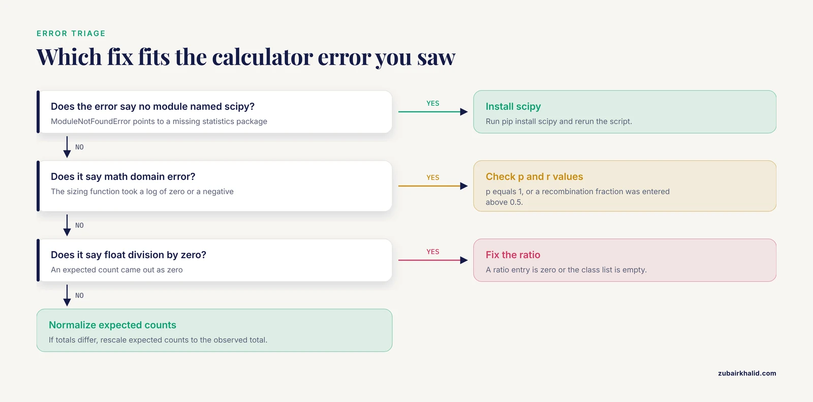
Three errors cover most runs:
ModuleNotFoundError: No module named 'scipy'means the statistics package is missing. Runpip install scipyand rerun the script.ValueError: math domain errorfrom the population sizing function means the code tried to take the logarithm of zero or a negative number. That happens when p equals 1, which would make the target class certain, or when a recombination fraction was entered above 0.5. Recombination fractions cannot exceed 0.5, so check the inputs.ZeroDivisionError: float division by zeroin the chi-square function means an expected count of zero, which happens when a ratio entry is zero or the class list is empty. Every class in the expectation needs a positive count.
A fourth failure is quiet rather than loud. If the observed and expected counts do not sum to the same total, some implementations raise an error and others silently rescale, so normalize the expected counts by the observed total before computing, as the helper function above does.
Worked Example: Marker-Assisted Backcrossing for Rice Aroma
Rice aroma shows every step above operating inside one real pipeline. The aroma of premium rice varieties comes from accumulation of 2-acetyl-1-pyrroline (2-AP), which results from loss-of-function mutations in the BADH2 gene. A published framework for aroma-focused breeding lays out the full sequence: high-quality DNA extraction, precise locus amplification and sequencing, variant discovery, conversion of polymorphisms into diagnostic markers, high-throughput genotyping, and systematic integration into crossing and selection programs [1].
The calculator slots into that sequence at three points. Foreground selection uses a functional marker inside BADH2 to keep BC1 plants carrying the nonfunctional aroma allele, and the 1:1 expectation from Step 3 says roughly half of each backcross progeny set qualifies before selection. Background selection (keeping progeny with recurrent parent alleles across the rest of the genome) pushes recovery beyond the 1 - (1/2)^n baseline, and the double recombinant formula from Step 5 sizes the population needed to find plants carrying the aroma allele with recurrent alleles on both sides. Codominant discrimination matters at both points, because heterozygotes must be told apart from homozygotes, and high-throughput SNP and KASP (Kompetitive Allele-Specific PCR) genotyping platforms make the required plant counts practical. The same framework supports rapid introgression into elite cultivars and gene pyramiding with other agronomic traits [1].
The worked numbers translate directly. Flanking markers at r = 0.10 mean screening roughly 600 BC1 plants to find one double recombinant, and three generations of backcrossing lift the background from 75% to about 94% recurrent genome before background selection pushes it higher.
Checking Your Results Against Real Genotype Data
Calculator output is a set of expectations, and three checks from the primary literature show how real data behave around those expectations.
Check the pedigree before trusting the labels. Molecular genotypes let you test for Mendelian inconsistencies, which flag individuals whose pedigree and genotype information disagree. In a selected Australian Angus cattle population of 11,224 animals genotyped for 61,105 autosomal markers, the additive genomic relationship between parent-offspring pairs, expected to be 0.5, averaged 0.488 with a standard deviation of 0.037, and full-sib pairs averaged 0.483 with a standard deviation of 0.054 [3]. The lesson for backcross work is that realized relatedness wobbles around the theoretical value. A BC1 plant whose genomic relationship to the recurrent parent lands slightly below 0.75 is not automatically mislabeled, so run the inconsistency check before discarding it.
Measure donor contribution instead of assuming it. In potato, researchers crossed the tetraploid cultivar Cooperation 88 with the diploid inducer IVP101, screened the diploid offspring by flow cytometry, and used SNP data to compute a theoretical introgression index. The inducer's nuclear genome persisted in some offspring, showing it was not completely eliminated during the wide hybridization [4]. The parallel for backcross planning is that residual donor genome is an empirical quantity, and marker-based indices catch what generation formulas miss.
Use backcross families to estimate parameters, not just count ratios. Backcross populations also feed variance component calculations. A pepper study crossed high androgenesis-response lines (androgenesis is the production of haploid plants from anther culture) with a non-responsive accession and phenotyped the parents, F1, F2, BC1P1, and BC1P2 generations. Broad-sense heritability (H², the share of trait variation from all genetic effects) came out at 0.96 to 0.97, narrow-sense heritability (h², the additive share that responds to selection) at 0.20 to 0.65, and the estimated gene number at 1.96 to 2.46, with additive effects accounting for 21% of gene action and dominance effects 79% [5]. When a backcross calculator includes heritability or gene number modules, those are the inputs and outputs involved.
Common Mistakes and Limitations
Individual crosses can behave atypically, so treat every calculator output as a plan to verify with marker data rather than a guarantee. Beyond that, eight mistakes account for most wrong answers.
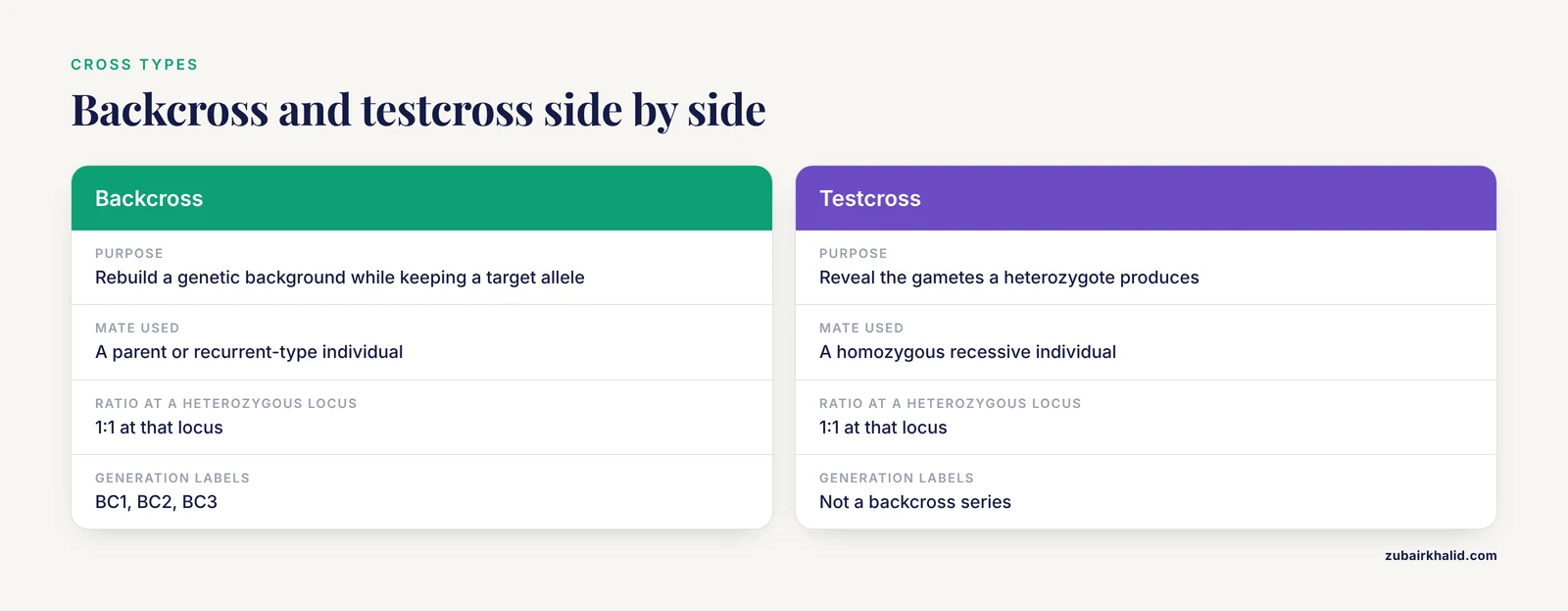
- Confusing a backcross with a testcross. A testcross mates a heterozygote to a homozygous recessive individual to reveal the gametes it produces. A backcross mates a hybrid back to a parent or recurrent-type individual to rebuild a genetic background. The ratios look similar (both give 1:1 at a heterozygous locus), but the goals differ, and calculators often label the two modes separately.
- Miscounting generations. The recovery formula 1 - (1/2)^n uses n backcross generations. Calling the F1 a backcross generation shifts every number by a factor of two. Label records BC1, BC2, BC3 and match the calculator's generation field to those labels.
- Treating expectations as guarantees. The 93.75% figure after three backcrosses is a population average. Individual plants range widely around it, which is exactly why background selection with markers exists, and realized genomic relationships drift slightly below theoretical values even in well-recorded pedigrees.
- Ignoring linkage. Unlinked-locus math gives clean 1:1:1:1 ratios, but linked loci distort them. Crossing over reshuffles allele combinations in ways that can add or subtract genetic variance, and in maize and wheat populations the measured contribution of crossing over to genetic variance ranged from positive 7% and 16% in two populations to strongly negative values between -74% and -25% in five others [6]. If your target and markers sit close together, use the (r1 × r2) / 2 calculation rather than independent assortment.
- Applying diploid formulas to polyploids. Standard backcross calculators assume two allele copies per locus. Polyploid crops carry more than two copies of each chromosome set, so a locus can hold three or more allele copies. In citrus tetraploids, inheritance depends on genome pairing behavior, and researchers estimate preferential pairing rates and parental heterozygosity restitution from marker data to separate disomic from tetrasomic segregation [7]. A diploid calculator will misstate genotype frequencies for these materials.
- Assuming the donor genome disappears completely. Residual donor DNA can persist beyond what generation counts predict, as the potato introgression work above demonstrated. Verify with genome-wide markers whenever the residual donor segment matters, for example when it carries linked deleterious alleles.
- Skipping the goodness-of-fit test. Counts that look close to 1:1 can still reject the expectation. Compute the chi-square and compare it against the critical value for the correct degrees of freedom. For two-locus expectations with four classes, use three degrees of freedom and the 7.815 critical value.
- Undersizing populations for rare classes. A double recombinant proportion of 0.005 needs hundreds of plants, not dozens. Run the sizing formula before planting, not after.
Tips for Getting More From Your Backcross Calculator
Fix the linkage phase first. Everything downstream depends on whether the F1 carries donor alleles in coupling or repulsion. Write the two F1 haplotypes at the top of your worksheet before any calculation.
Choose codominant markers and enough of them. Codominant markers distinguish all three genotypes at a locus, which foreground and background selection both require. High-throughput SNP platforms such as KASP make it practical to screen the hundreds of plants that double recombinant sizing demands [1].
Use population-specific recombination data when you can. The contribution of crossing over differs sharply between populations and traits, as the maize and wheat results in the mistakes section show, so a target interval inherited in one background can behave differently in another. A generic map distance is a starting point, not a final input.
Balance gain against diversity. Backcrossing concentrates a program on one recurrent background, and intense selection on top of that narrows diversity further. Optimal contribution selection, which optimizes parental contributions to maximize genetic gain while controlling the rate of inbreeding, is the framework breeders use to avoid the vigor losses of inbreeding depression [8]. Your calculator can flag the risk by tracking cumulative family contributions across cycles.
Collect the inputs for population-level calculations early. When results from several biparental populations feed one program, a framework for estimating genetic covariance between populations requires marker effects for each population, a linkage map, linkage phase information, and the inbreeding coefficient of the populations [9]. Those four inputs are worth recording from the first generation.
Handle unbalanced pedigree data with mixed models. Long-running programs accumulate messy records. A 30-year almond breeding dataset covering more than 17,500 individuals used Bayesian linear mixed models, implemented in the MCMCglmm R package, to estimate breeding values and variance components even for individuals without phenotypic records, with repeatability estimates ranging from 0.15 to 0.56 across traits [10]. The same modeling approach extends a backcross calculator from simple ratios to breeding value estimation.
A sensible next step is to rerun the six steps with your own cross parameters, then verify the plan against marker data as each generation is genotyped.
Frequently Asked Questions
What is a backcross calculator in genetics?
A backcross calculator is a tool that computes the genotype frequencies, genome recovery percentages, population sizes, and goodness-of-fit statistics that repeated backcrossing produces. It turns the halving rule of backcross genetics into numbers you can plan a crossing program around.
How much recurrent parent genome returns after each backcross generation?
The expected fraction is 1 - (1/2)^n, which gives 75% after one backcross, 87.5% after two, 93.75% after three, and about 99.2% after six. Marker-based background selection can push recovery above these averages.
How many progeny do I need to recover a specific recombinant genotype?
Use N ≥ ln(1 - c) / ln(1 - p), where p is the proportion of the target genotype and c is your confidence level. For a double recombinant class at p = 0.005 and 95% confidence, screen 598 progeny.
What is the difference between a backcross and a testcross?
A testcross mates a heterozygote to a homozygous recessive individual to reveal the gametes it produces. A backcross mates a hybrid back to a parent or recurrent-type individual to rebuild that parent's genetic background while keeping a target allele.
How do I test whether my backcross counts fit a 1:1 ratio?
Compute chi-square as Σ (O - E)² / E with one degree of freedom. Counts of 52 and 48 give χ² = 0.16, well below the 3.841 critical value, so the 1:1 expectation stands.
Can backcross calculators handle polyploid crops?
Standard diploid calculators cannot, because polyploids carry more than two allele copies per locus and may show disomic or tetrasomic segregation. Use tools that model pairing behavior and estimate heterozygosity restitution from marker data.
What are foreground and background selection?
Foreground selection keeps progeny that carry the donor allele at the target locus. Background selection keeps progeny with recurrent parent alleles across the rest of the genome, which accelerates recovery beyond the 1 - (1/2)^n baseline.
Do backcross calculations account for linkage?
Basic calculators assume independent assortment. For linked markers, use the double recombinant proportion (r1 × r2) / 2 and size the population accordingly, because linkage changes which genotype classes appear and how often.
Sources
- Application of Molecular Markers for Trait-Specific Breeding of Aroma Accumulation in Rice.
- Genetic analysis of pericarp pigmentation variation in Corn Belt dent maize.
- Short communication: genomic kinship, opposing homozygotes and genetic diversity in a selected population of Australian Angus cattle.
- Genetic characteristics of the diploid offsprings in potato Cooperation 88 induced by diploid donor IVP101.
- Inheritance of androgenesis response in pepper.
- Contribution of crossing over to genetic variance in maize and wheat populations.
- Inheritance pattern of tetraploids pummelo, mandarin, and their interspecific hybrid sour orange is highly influenced by their phylogenomic structure.
- Balancing gain and diversity: Optimal contribution selection for sustainable genetic improvement in sugarcane.
- Genetic covariance between plant biparental populations: concept and estimation.
- Genetic evaluation of flowering, maturity time and productivity in almond (Prunus dulcis): heritability estimates and breeding value predictions.